Nonlinear statistical models. Ch. 1, Univariate nonlinear regression.

•

by

A. Ronald Gallant

CHAPTER 1. Univariate Nonlinear Regression

com~ents

and report errors to the followins address.

A. Ronald Gallant

Institute of Statistics

North Carolina State University

Posl Office Box 5457

Raleish,

Ne

27650

USA

Phone: 1-919-737-2531

Additional copies Day be ordered

fro~

the Institute of Statistics al a

price of $15.00 for USA delivery; additional postaSe will be charSed for

overseas orders.

NONLINEAR STATISTICAL MODELS

Table of Contents

1.

Univariate Nonlinear Regression

1.0

Preface

1.1

Introduction

1.2

Taylor's Theorem and Matters of Notation

1.3

Statistical Properties of Least SQuares

Estimators

1.i

Methods of Computing Least SQuares Estimators

1.5

HYPothesis Testing

1.6

Confidence Intervals

1.7

References

1.B

Inde>:

2.

Univariate Nonlinear Regression:

Special Situations

3.

A Unified

Asy~ptotic

Theory of Nonlinear Statistical

Models

3.0

Preface

3.1

Introduction

3.2

The Data Generating Model and Limits of Cesaro

Sums

3.3

Least Mean Distance Esti.ators

3.i

Method of MaRlen ts Estimators

3.5

Tests of HYPotheses

3.6

Alternative Representations of a HYPothesis

3.7

Rando. Regressors

3.B

Constrained Estimation

3.9

References

3.10

Index

4.

Univariate Nonlinear Regression:

AsYmptotic Theory

5.

Multivariate Linear Models:

Review

6.

Multivariate Nonlinear Models

7.

Linear Simultaneous EQuations Models:

Review

8.

Nonlinear Simultaneous EQuations Models

CHAPTER 1. Univariate Nonlinear Regression

The nonlinear regression model with a univariate dependent variable is more frequently used in applications than any of the other methods discussed in this book. Moreover, these other methods are for the most part fairly straightforward extensions of the ideas of univariate nonlinear regression. Accordingly, we shall take up this topic first and consider it in some detail.

In this chapter, we shall present the theory and methods of univariate nonlinear regression by relying on analogy with the theory and methods of linear regression, on examples, and on Monte-Carlo illustrations. The formal mathematical verifications are presented in subsequent chapters. The topic lends itself to this treatment as the role of the theory is to justify some intuitively obvious linear approximations derived from Taylor's expansions. Thus one can get the main ideas across first and save the theoretical details until later. This is not to say that the theory is unimportant. Intuition is not entirely reliable and some surprises are uncovered by careful attention to regularity conditions and mathematical detail.

As a practical matter, the computations for nonlinear regression methods must be performed using either a scientific subroutine library such as IMSL or NAg Libraries or a statistical package with nonlinear capabilities such as SAS, BMDP, TROLL, or TSP. Hand calculator computations are out of the question. One who writes his own code with repetitive use in mind will probably produce something similar to the routines found in a scientific subroutine library. Thus, a scientific subroutine library or a statistical package are effectively the two practical alternatives. Granted that

scientific subroutine packages are far more flexible than statistical packages and are usually nearer to the state of the art of numerical analysis than the

1. INTRODUCTION

One of the most common situations in statistical analysis is that of data which consist of observed, univariate responses Yt known to be dependent on corresponding k-dimensional inputs xt • This situation may be represented by the regression equations

t - 1,2, •••,n

where f(x,e) is the known response function, eO is a p-dimensional vector of unknown parameters, and the e t represent unobservable observational or

experimental errors. We write eO to emphasize that it is the true, but unknown, value of the parameter vector e that is meant; e itself is used to denote instances when the parameter vector is treated as a variable as, for instance, in differentiation. The errors are assumed to be independently and identically distributed with mean zero and unknown variance a2• The sequence of independent variables {xtl is treated as a fixed known sequence of

constants, not random variables. If some components of the independent vectors were generated by a random process, then the analysis is conditional on that realization {x

t } which obtained for the data at hand. See Section 2 of the next chapter for additional details on this point and Section 7 of the next chapter in which is displayed a device that allows one to consider the random regressor set-up as a special case in a fixed regressor theory.

1-1-2

By exploiting various transformations of the independent and dependent variables, viz.

the scope of models that are linear in the parameters can be extended

considerably. But there is a limit to what can be adequately approximated by a linear model. At times a plot of the data or other data analytic

considerations will indicate that a model which is not linear in its

parameters will better represent the data. More frequently, nonlinear models arise in instances where a specific scientific discipline specifies the form that the data ought to follow and this form is nonlinear. For example, a response function which arises from the solution of a differential equation might assume the form

Another example is a set of responses that is known to be periodic in time but with an unknown period. A response function for such data is

A univariate nonlinear regression model is of the form

but since the transformation ~O can be absorbed into the definition of the dependent variable, the model

is sufficiently general. Under these definitions a linear model is a special case of the nonlinear model in the same sense that a central chi-square

distribution is a special case of the non-central chi-square distribution. This is somewhat of an abuse of language as one ought to say regression model and linear regression model rather than nonlinear regression model and

(linear) regression model to refer to these two categories. But this usage is long established and it is senseless to seek change now.

EXAMPLE 1. The example that we shall use most frequently in illustration has the response function

and the vector valued parameter is

6 •

so that for this response function k • 3 and p ,.. 4. A set of observed responses and inputs for this model which will be used to illustrate the computations is given in Table 1. The inputs correspond to a one-way "treatment-control" design that uses experimental material whose age (ax3) affects the response exponentially. That is, the first observation

Xl • (0,1,6.28)

represents experimental material with attained age x3 ,.. 6.28 months that was (randomly) allocated to the control group and has expected response.

o 6.286

3

f ( 60 ) 60

2

+

6

0

4 e xl' ,..

Similarly, the second observation

X

2 • (1,1,9.86)

Table l- Oa ta Va 1 ues fo r Examp1 e 1.

e

t y _{Xl X2 X3}

1 0.98610 1 1 6.28

2 1.03848 0 1 9.86

3 0.95482 1 1 9.11

4 1. 04184 0 1 8.43

5 1.02324 1 1 8.11

6 0.90475 0 1 1.82

7 0.96263 1 1 6.58

8 1.05026 0 1 5.02

9 0.98861 1 1 6.52

10 1.03437 0 1 3.75

11 0.98982 1 1 9.86

12 1.01214 0 1 7.31

13 0.66768 1 1 0.47

14 0.55107 0 1 0.07

15 0.96822 1 1 4.07

16 0.98823 0 1 4.61

17 0.59759 1 1 0.17

18 0.99418 0 1 6.99

19 1.01962 1 1 4.39

20 0.69163 0 1 0.39

21 1. 04255 1 1 4.73

22 1.04343 0 1 9.42

23 0.97526 1 1 8.90

24 1.04969 0 1 3.02

25 0.80219 1 1 0.77

26 1.01046 0 1 3.31

27 0.95196 1 1 4.51

28 0.97658 0 1 2.65

29 0.50811 1 1 0.08

and so on. The parameter 6~ is, then, the treatment effect. The data of Table 1 are simulated.

EXAMPLE 2. Quite often, nonlinear models arise as solutions of a system of differential equations. The following linear system has been used so often in the nonlinear regression literature (Box and Lucus (1959), Guttman and Meeter (1964), Gallant (1980» that it might be called the standard

pedagogical example. Linear System

(d/dx)A(x) • -6₁A(x)

(d/dx)C(x) - 6 2B(x) Boundary Conditions

A(x) - 1, B(x) - C(x)

=

0 at time x

=

0 Parameter Space

Solution, 6

1

>

62 -6

x

A(x) • e 1

-6

x

C(x) • 1 - (6

1 - 62)-1(61e 2

-6 x

1

- 6 e )

A(x) • Solution, 6

1 • 62 -6

1x

e

C(x)

Systems such as this arise in compartment analysis where the rate of flow of a substance from compartment A into compartment B is a constant proportion

61 of the amount A(x) present in compartment A at time x. Similarly, the rate of flow from B to C is a constant proportion 62 of the amount B(x) present in compartment B at time x. The rate of change of the quantities within each compartment is described by the system of linear differential equations. In chemical kinetics, this model describes a reaction where substance A

decomposes at a reaction rate of 61 to form substance B which in turn decomposes at a rate 62 to form substance C. There are a great number of other instances where linear systems of differential equations such as this arise.

Model B

f(x,6)

-o

6 .. (1.4, .4)

{X

t } - {.2S, .5, 1, 1.5, 2,

4,

.25, .5, 1, 1.5, 2,

4}

n - 12

2 2

a .. (.025)

Model C

f(x,6) •

-x6

2 -x61

1 - (6

1e - 62e )/(61 - 62) -x6

1 -x61

1 - e - xt3 e

1

60 • (1.4, .4)

{X

t } • {I, 2, 3, 4, 5, 6, 1, 2, 3, 4, 5, 6}

Table 2. Data Values for Example 2.

t Y X

Model B

1 0.316122 0.25

2 0.421297 0.50

3 0.601996 1.00

4 0.573076 1. 50

5 0.545661 2.00

6 0.281509 4.00

7 0.273234 0.25

8 0.415292 0.50

9 0.603644 1.00

10 0.621614 1.50

11 0.515790 2.00

12 0.278507 4.00

Model C

1 0.137790 1

2 0.409262 2

3 0.639014 3

4 0.736366 4

5 0.786320 5

6 0.893237 6

7 0.163208 1

8 0.372145 2

9 0.599155 3

10 0.749201 4

11 0.835155 5

2. TAYLOR'S THEOREM AND MATTERS OF NOTATION

In what follows, a matrix notation for certain concepts in differential calculus leads to a more compact and readable exposition. Suppose that s(6) is a real valued function of a p-dimensional argument 6. The notation

(a/a6)s(6) denotes the gradient of s(6),

(an 6

1)s(6) (a/aS

2)s(S)

p 1

a p by 1 (column) vector with typical element (a/a6

i )s(6). Its transpose is denoted by

,

(a/a6 )s(6) = [(a/a6

1)s(6), (a/a62)s(6), ••• , (a/aSp)s(6)]

1 p

Suppose that all second order derivatives of s(6) exist. They can be arranged in a p by p matrix, known as the Hessian matrix of the function s(6),

(a2/ as i)s(6)

2

(a /as

2as1)s(S)

2

(a /as

1aS2)s(6)

(a2/as~)s(s)

...

(a2/ as1 a6_p)s(6) (a2/a6

2a6p)s(6)

If the second order derivatives of s(8) are continuous functions in 8 then the Hessian matrix is symmetric (Young's theorem).

Let f(8) be an n by 1 (column) vector-valued function of a p-dimensional argument 8. The Jacobian of

f(8) •

n 1

is the n by p matrix

(3/a8

1)f1(8) (a/a8

1)f2(8)

,

(a/a8 )f(8)

=

(a/a8

2)f1(8) (a/38

2)f2(8)

(a/a8

p)f1(8) (a/a8

p)f2(8)

n

,

Let h (8) be an n by 1 (row) vector-valued function

(a/a8 )f (8)

P

n

Then

1-2-3

,

(a/aa)h (a) •

(a/aa

1)h1(a) (3/aa

2)h1(a)

(a/aa

1)hZ(a) ••• (a/aa

_z

)h

2(a)

(a/aa

1)hn(a) (a/aaZ)hn(a)

p

(a/aa )h (a)

p n

n

In this notation, the following rule governs matrix transposition:

,

,

[(a/a6 )f(a)]

=

(a/aa)f (a)

And the Hessian matrix of s(a) can be obtained by successive differentiation variously as:

=

(a/aa)[(a/aa)s(6)]

,

=

(a/aa )[(a/aa)s(a)]

,

,

,

=

(a/a6 )[(a/aa )s(a)]

(if symmetric)

(if symmetric)

One has a chain rule and a composite function rule. They read as follows. If

,

f(6) and h (a) are as above then (Problem 1)

,

,

,

,

,

,

(a/a6 )h (6)f(a)

=

h (6)[(a/aa )f(a)]

+

f (6)[(a/a6 )h(6)]

Let g(p) be a p by 1 (column) vector-valued function of a r-dimensional argument p and let f(6) as above: Then (Problem 2)

t t t

(a/ap )f[g(p)] m

(a/a6

)f(6)!6-g(p) (a/ap )g(p)

n p r

The set of nonlinear regression equations

t"'1,2, •••,n

may be written in a convenient vector form

by adopting conventions analogous to those employed in linear regression; namely

Y1 Y2 Y •

Yn

1-2-5

f(x 1, a) f(x

2,a) f(a) ..

···

f(x ,a) n

n 1

e 1 e

2

·

e

-··

e

n

n 1

The sum of squ~red deviations

SSE(a) =

of the observed Yt from the predicted value f(xt,a) corresponding to a trial value of the parameter a becomes

, 2

SSE(a) = [y - f(a)] [y - f(a)] .. Uy - f(a)U

in this vector notation.

The estimators employed in nonlinear regression can be characterized as linear and quadratic forms in the vector e which are similar in appearance to those that appear in linear regression to within an error of approximation that becomes negligible in large samples. Let

,

that is, F(6) is the matrix with typical element (a/a6

j )f(xt ,6) where t is the

~

row index and j is the column index. The matrix F(60) plays the same role in

these linear and quadratic forms as the design matrix X in the linear regression.

z •

xa

+

e.

The appropr ate ana ogyi 1 is ° ta neb i d by sett ng z • y -i f(6 0) + F(60)6° and setting X • F(60). Malinvaud (1970, Ch. 9) terms this equation the "linear pseudo-model." For simplicity we shall write F for the matrix F(6) when it is evaluated at 6.6°;

Let us illustrate these notations with Example 1.

EXAMPLE 1 (continued). Direct application of the definitions of y and f(6) yields

0.98610 1.03848 0.95482

y = 1.04184

0.50811 0.91840

f(6)

=

30

Since

6.286 3 6

1 + 62 + 64e 9.866

3

6

2

+

64e

9.116 3 6

1

+

62

+

64e

8.436₃

6

2

+

64e

0.086 3 6

1

+

62

+

64e 6.116

3

6

2

+

64e

1

1 1

6.286

3 6.2863 6₄(6.28)e e

0 1

9.866

3 9.8663 6

4(9.86)e e

1 1

9.116

3 9.1163 6

4(9.11)e e

F(6) • 0 1

8.436

3 8.4363 6

4(8.43)e e

1 1

. 0.086

3 0.0863 6

4(0.08)e e

0 1

6.116

3 6.1163 6

4(6.11)e e

30 4

Taylor's theorem, as we shall use it, reads as follows:

Taylor's Theorem: Let s(6) be a real valued function defined over 0. Let 0 be an open, convex subset of RP; RP denotes p-dimensional Euclidean space. Let 60 be some point in 0.

If s(6) is once continuously differentiable on 0 then

or, in vector notation,

If s(a) is twice continuously differentiable on

e

then

or t in vector notation t

for some

e

=

xao

+

(I-X)a where 0 ~ X~ 1.

Applying Taylor's theorem to f(x tt a) we have

implicitly assuming that f(x,a) is twice continuously differentiable on some open t convex set

e.

Note that e is a function of both x and at e

=

e(x,e). Applying this formula row by row to the vector f(e) we have the approximation

where a typical row of R is

Using the previous formulas,

,

,

,

(a/a6 )SSE(6) - (a/a6 )[y - f(6)] [y - f(6)]

,

,

,

,

• [y - f(6)] (a/a6 )[y - f(6)]

+

[y - f(6)] (a/a6 )[y - f(6)]

,

,

• 2[y - f(6)] [-(a/a6 )f(6)]

,

- -2[y - f(6)] F(6)

The least squares estimator is that value 6 that minimizes SSE(6) over the parameter space

a.

If SSE(6) is once continuously differentiable on some open set

eo

with 6 e:

rJ>

a,

then 6 satisfies the "normal equations"

,

...

F (6)[y - f(6)] = O.

This is because (a/a6)SSE(6) - 0 at any local optimum. In linear regression,

z •

xa

+

e,

least square residuals e computed as

e •

y - xa,

, A X e = O.

In nonlinear regression, least squares residuals are orthogonal to the columns of the Jacobian of f(6) evaluated at 6 - 6, viz.,

, A

PROBLEMS

1. (Chain rule). Show that

,

,

,

,

,

,

(a/ae )h (e)f(e) • h (e)(a/ae )f(e)

+

f (e)(a/ae )h(e)

n

by computing (a/ae

i )

L

~(e)fk(e) by the chain rule for ia 1,2, ••• ,p to obtain

k-1

, , n , n ,

(alae

)h (e)f(e).

L

~(e)(a/ae )fk(e)

+

L

fk(e)(a/ae )~(e)

ka_{1 k-1}

,

,

Note that (alae )fk(e) is the k-th row of

(alae

)f(e).

2. (Composite function rule). Show that

,

,

,

(a/ap

)f[g(P)]

=

{(alae )f[g(p)]}(a/ap)g(p)

,

3. STATISTICAL PROPERTIES OF LEAST SQUARES ESTIMATORS

The least squares estimator of the unknown parameter 60 in the nonlinear model

o

y "" f(6 )

+

e

is the p by 1 vector 6 that minimizes

I 2

SSE(6) "" [y - f(6)] [y - f(6)] "" lIy - f(6) II •

The estimate of the variance of the errors e t corresponding to the least squares estimator 6 is

In Chapter 4 we shall show that

.. 0

' - 1 '

6 "" 6

+

(F F) F e

+

0 (1/1n) p

2 I , - 1 '

s "" e [I - F(F F) F ]e/(n-p)

+

0 (l/n)

p

o ' 0

where, recall, F "" F(6 ) "" (a/a6 )f(6 ) "" matrix with typical element

, 0

(a/a6 )f(xt,e). The notation 0 (a ) denotes a (possibly) matrix-valued p n

random variable X "" 0 (a ) with the property that each element ~jn satisfies

n p n

lim p[IX_ij /a

I >

€] "" 0

for any €

>

0; {a } is some sequence of real numbers. the most frequent n

choices being a_n

=

1. a_n • 1/1n. and a_n - l/n.

These equations suggest that a good approximation to the joint .... 2

distribution of (a.s ) can be obtained by simply ignoring the

terms 0 (1/10) and 0 (l/n). Then by noting the similarity of the equations

p p

.... ' 1 '

a - aO

+

(F F) - F e

with the equations that arise in linear models theory and assuming normal errors we have approximately that a has the p-dimensional multivariate normal

o 2 ' -1

-distribution with mean a and variance-covariance matrix a (F F) ; ~

(n-p)s2/ a2 has the chi-squared distribution with (n-p) degrees of freedom.

2 2 2

(n-p)s

/a

,."

X (n-p);

2 .... .... 2

1-3-3

The alternative to this method of obtaining an approximation to the

distribution of 6--characterization coupled with a normality assumption--is to use conventional asymptotic arguments. One finds that 6 converges almost surely to 60, s2 converges almost surely to 02 , (1/n)F'(6)F(6) converges

" 0

almost surely to a matrix

n,

and that

10(6 -

6 ) is asymptotically normally distributed as the p-variate normal with mean zero and variance-covariance matrix 020-1,

" L 2 -1

1n(6 - 60) -+ N (0,0 0 ).

p

The normality assumption is not needed. Let

,

"

o =

(1/n)F (6)F(6).

Following the characterization/normality approach it is natural to write

Following the asymptotic normality approach it is natural to write

2 "

( =

N (O,s nC) );

p

natural perhaps even to drop the degrees of freedom correction and use

"2

to estimate 02 instead of s2. The practical difficulty with this is that one

can never be sure of the scaling factors in computer output. Natural combinations to report are:

a,

s2

,

c;

A _{2 2}A

a,

s

,

s

c;

a,

o ,A2

o .

A_1

,

a,

o ,A2 0A2 A_1

o .

,

and so on. The documentation usually leaves some doubt in the reader's mind as to what is actually printed. Probably, the best strategy is to run the program using Example 1 and resolve the issue by comparison with the results reported in the next section.

As in linear regression, the practical importance of these distributional properties is their use to set confidence intervals on the unknown parameters

a~ (i~1,2,••• ,p) and to test hypotheses. For example, a 95% confidence interval may be found for a~ _{from the .025 critical value t. 025 of the} t-distribution with n-p degrees of freedom as

o

*

Similarly, the hypothesis H:

a

-with It.02S

1

and rejecting H when Itil

>

It._02S

I;

c_ii denotes the i-th

diagonal element of the matrix C. The next few paragraphs are an attempt to convey an intuitive feel for the nature of the regularity conditions used to obtain these results; the reade~ is reminded once again that they are

presented with complete rigor in Chapter 4.

The sequence of input vectors {x_t } must behave properly as n tends to infinity. _{Proper behavior is obtained when the components Xit of xt are} chosen either by random sampling from some distribution or (possibly

disproportionate) replication of a fixed set of points. In the latter case, some set of points aO' al, ••• ,aT-l is chosen and the inputs assigned according to Xit

=

aCt mod

T)·

Disproportionality is accomplished by allowing some of the ai to be equal. More general schemes than these are permitted--see

Section 2 of Chapter 3 for full details--but this is enough to gain a feel for the sort of stability that {x

t} ought to exhibit. Consider, for instance, the data generating scheme of Example 1.

EXAMPLE 1 (continued). The first two coordinates Xlt' X2t of

,

xt

=

(xlt' X2t' X3t) consist of replication of a fixed set of design points determined by the design structure:

(X

1

,X

2)1 (x₁,x₂)2

(x

1,X2)t

(x₁'X₂)t

-=

-(1,1), (0,1),

(1,1),

(0,1),

That is,

with

•

a_{(t mod 2)}

•

•

(0,1),

(1,1)

(a/aai)f(x,a) must be

2

(a /aa

i aaj )f(x, a) 1Il1st

The covariate X3t is the age of the experimental material and 1s conceptually a random sample from the age distribution of the population due to the random allocation of experimental units to treatments. In the simulated data of Table 1, X3t was generated by random selection from the uniform distribution on the interval [0,10]. In a practical application one would probably not know the age distribution of the experimental material but would be prepared

to assume that x3 was distributed according to a continuous distribution function that has a density P3(x) which is positive everywhere on some known interval [O,b], there being some doubt as to how much probability mass was to the right of b.

I

The response function f(x,a) must be continuous in the argument (x,a); that is, if lim (xi,a

i) - (x*,a*) (in Euclidean norm on Rk+P) then

i+GO

* *

lim f(xi,a

i) - f(x ,a). The first partial derivatives

i+GO

continuous in (x,a) and the second partial derivatives

be continuous in (x, a). These smoothness requirements are due to the heavy use of Taylor's theorem in Chapter 3. Some relaxation of the second

There remain two further restrictions on the limiting behavior of the response function and its derivatives which roughly correspond to estimabi1ity considerations in linear models.

s(e) • lim

(lIn)

n~

The first is that

n

I

[f(xt,e) - f(x t,e

O )]2

tal

has a unique minimum at e

=

eO and the second is that the matrix

g • lim (l/n)F' (eo)F(eo ) n~

be non-singular. We term these the Identification Condition and the Rank Qualification respectively. When random sampling is involved, Kolmogorov's Strong Law of Large Numbers is used to obtain the limit as we illustrate with Example 1, below. These two conditions are tedious to verify in applications and few would bother to do so. However, these conditions indirectly impose restrictions on the inputs xt and parameter 60 that are often easy to spot by inspection. Although 60 is unknown in an estimation situation, when testing hypotheses one should check whether the null hypothesis violates these

assumptions. If this happens, methods to circumvent the difficulty are given in the next chapter. For Example 1, either H: 6o 0

3 - 0 or H: 64

=

0 will violate the Rank Qualification and the Identification Condition as we next show.

EXAMPLE 1 (continued). We shall first consider how the problems with H: 6~ • 0 and H: 6~ • 0 can be detected by inspection, next consider how limits are to be computed, and last how one verifies that

n 0 2

s(6)

=

lim

(lIn)

I

[f(x

t ,6) - f(xt ,6)] has a unique minimum at 6 = 6

0 •

Consider the case H: aO

.. °

leaving the case H: aO

.. °

to Problem 1• I f

3 4

aO

- °

_then 3

1 1 _a4x31 1

°

1 _a4x32 1

1 1 _a4x33 1

F(a) -

_°

1 _a4x34 1

..

1 1 _a4x3n-1 1

°

1 _{a 4x3n} 1

F(a) has two columns of ones and is, thus, singular. Now this fact can be noted at sight in applications; there is no need for any analysis. It is this kind of easily checked violation of the regularity conditons that one should guard a~ainst. Let us verify that the singularity carries over to the

limit. Let

, n

G (a) - (l/n)F (a)F(a) - (l/n)

I

[(a/aa)f(x ,a)][(a/aa)f(x ,a)]

n t-1 t t

The regularity conditions of Chapter 4 guarantee that lim G (a) exists and we

n+oo n

,

shall show it directly below. Put

A -

(0,1,0,-1). Then

, n , 2

A

Gn(a)1

A -

(l/n)

I

[A

(a/aa)f(xt,a)! ] - 0.

a

-0 t-1

a

-0

3 3

,

,

Since zero for every n,

A

[lim Gn(a)l

]A ..

°

by continuity of

A AA

in

A.

n+ClO

a

-0

3 Recall that {x

continuous function g(x) we must have f~lg(x)lp3(x)dx

<

~ so that by Ko1mogorov's Strong Law of Large Numbers (Tucker, 1967)

n

lim (l/n)

L

g(x_3t) ,. f~g(x)P3(x)dx no+<» t-1

Applying these facts to the treatment group we have

n

lim (2/n)

L

[f(xt,S) - f(x

t ,SO)]2 no+<» todd

Applying them to the control group we have

lim (2/n) no+<»

n

L

[f(xt,S) - f(x

t,SO)]2 t even

Then

and we let F3(x3) be the distribution function corresponding to P3(x). Let

(1,1)

f

[f(x,6) - f(x,6 )]0 2d~(z) • (1/2) '\L -,cJO[f(x,6) - f(x,6 )] P3(x)dx0 2 (x

1,x2)-(0,1)

where the integral on the left is a Lebesque-Stei1tjes integral (Royden, 1963, Ch. 12; or Tucker, 1967, Sec. 2.2). In this notation the limit can be given an integral representation

~

0 2

f

0 2

lim (l/n) L [f(x

t ,6) - f(xt,6)] - [f(x,6) - f(x,6 )] d~(x).

n+<» t-1

These are the ideas behind Section 2 of Chapter 3. The advantage of the integral representation is that familiar results from integration theory can be used to deduce properties of limits. As an example: What is required of f(x,6) such that

(a/ as) lim

n+<» n

L

f(x ,6) - lim

t-1 t n+<»

n

L

(a/aS)f(x

t,6)? t-1

We find later that the existence of b(x) with l(a/a6)f(x,6)1 ( b(x) and

fb(x)d~(x)

<

~ is enough given continuity of (a/a6)f(x,6).

Our last task is to verify that

f

0 2

=

0/2)

has a unique minimum. Since s(6) ) 0 in general and s(60)

=

0, the question is: Does s(6) = 0 imply that 6

=

6°? One first notes that 6~

=

0 or 6~ - 0 must be ruled out as in the former case any 6 with 6₃

=

0 and

°

°

6

2

+

64

=

62

+

64 will have s(6)

=

0 and in the latter case any 6 with

6

1

=

6~, 62

=

6~, 64

=

0 will have s(6) - O. Then assume that 6~

*

0 and

6~

*

0 and recall that P3(x)

>

0 on [O,b]. Now s(6)

=

0 implies

Differentiating we have

o

< x < b

6

3x 6°3x

6 6_{3 4}e _- 6°6°_{3 4}e

₌

0

o

<

x

<

b

Putting

x -

0 we have 6

364

=

6

° °

364 whence

o

<

x

<

b

°

which implies 6

3

=

63, We now have that

But if 6₃ • 6~, _{64 •} 6~, and s(6) • 0 then

which implies 6₁ • 6~ and 6₂ • 6~. In summary

s(6) • 0,

6~

*

0,

6~

*

0

->

6 . 60•

As seen from Example

I,

checking the Identification Condition and Rank Qualification is a tedious chore to be put to at every instance one uses nonlinear methods. Uniqueness depends on the interaction of f(x,6) and ~(x)

and verification is ad hoc. Similarly for the Rank Qualification (Problem 2). As a practical matter, one should be on guard against obvious problems

and can usually trust that numerical difficulties in computing 6 will serve as

~

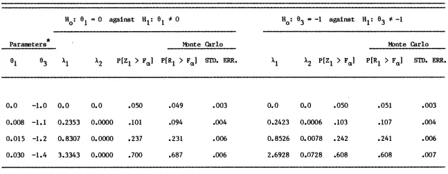
a sufficient warning against subtle problems as seen in the next section.

An appropriate question is how accurate are probability statements based on the asymptotic properties of nonlinear least squares estimators in

applications. Specifically one might ask: How accurate are probability

statements obtained by using the critical points of the t-distribution with n-p degrees of freedom to an-pn-proximate the samn-pling distribution of

Monte Carlo evidence on this point is presented below using Example 1. We shall accumulate such information as we progress.

Table 3. Enpirical DistribJtion of t

i Coupared to the t-distribJtion

1-3-13

Tabular Values Enpirical DistribJtion

-c p(t .. c) P(t

1 .. c) P(t2 ) c) P(t3 .. c) P(t4 .. c) Std. Error

-3.707 .0005 .0010 .0010 .0000 .0002 .0003

-2.779 .0050 .0048 .0052 .0018 .0050 .0010

-2.056 .0250 .0270 .0280 .0140 .0270 .0022

-1.706 .0500 .0522 .0540 .0358 .0494 .0031

-1.315 .1000 .1026 .1030 .0866 .0998 .0042

-1.058 .1500 .1552 .1420 .1408 .1584 .0050

-0.856 .200 .2096 .1900 .1896 .2092 .0057

-0.684 .2500 .2586 .2372 .2470 .2638 .0061

0.0 .5000 .5152 .4800 .4974 .5196 .0071

0.684 .7500 .7558 .7270 .7430 .7670 .0061

0.856 .8000 .8072 .7818 .7872 .8068 .0057

1.058 .8500 .8548 .8362 .8346 .8536 .0050

1.315 .9000 .9038 .8914 .8776 .9004 .0042

1.706 .9500 .9552 .9498 .9314 .9486 .0031

2.056 .9750 .9772 .9780 .9584 .9728 .0022

2.779 .9950 .9950 .9940 .9852 .9936 .0010

points of the t-distribution. The responses were generated using the inputs of Table 1 with the parameters of the model set at

,

eO _

(0, 1, -1, -.S) ,

02 - .001.

The standard errors shown in the table are the standard errors of an estimate of the probability p(t

<

c) computed from SOOO Monte Carlo trials assuming that t follows the t-distribution. If that assumption is correct, the Monte Carlo estimate of P[t

<

c] follows the binomial distributi~nand has variance

P(t

<

c) • p(t

>

c)/SOOO.

Table 3 indicates that the critical points of the t-distribution describe

~

the sampling behavior of t

i reasonably well. For example, the Monte Carlo estimate of the Type I error for a two-tailed test of H:

eO -

-1 using the

3

PROBLEMS

1. Show that H: e~ - 0 will violate the Rank Qualification in Example 1.

,

2. Show that Q - lim (l/n)F (e)F(e) has full rank in Example 1 if

n+co

4. METHODS OF COMPUTING LEAST SQUARES ESTIMATORS

The more widely used methods of computing nonlinear least squares

estimators are Hartley's (1961) modified Gauss-Newton method and the Levenberg (1944)-Marquardt (1963) algorithm.

The Gauss-Newton method is based on the substitution of a first order Taylor's series aproximation to f(8) about a trial parameter value 8T in the formula for the residual sum of squares SSE(8). The approximating sum of squares surface thus obtained is

The value of the parameter minimizing the approximating sum of squares surface is (Problem 1)

It would seem that ~ should be a better approximation to the least squares estimator 8 than 8T in the sense that SSE(8M)

<

SSE(8T). These ideas are displayed graphically in Figure 1 in the case that 8 is univariate (p=l).

As suggested by Figure 1, SSET(S) is tangent to the curve SSE(S) at the point ST. The approximation is first order in the sense that one can show that (Problem 2)

lim ISSE(S) - SSET(S)I/ns - ST" =

a

1-4-2

but not second order since the best one can show in general is that (Problem 2)

SSE

a

Figure 1. The Linearized Approximation to the Residual Sum of Squares Surface, an Adequate Approximation

a

It is not necessarily true that aM is closer to a than aT in the sense that

SSE

I i

a

Figure 2. The Linearized Approximation to the Residual Sum of Squares Surface, A Poor Approximation

a

But as suggested by Figure 2, points on the line segment joining aT to ~

that are sufficiently close to aT ought to lead to improvement. This is the

*

case and one can show (Problem 3) that there is a

A

such that all points with

*

o <

A

<

A

satisfy

1-4-4

These are the ideas that motivate the modified Gauss-Newton algorithm which is as follows:

0)' Choose a starting estimate 6₀• Compute

D • [F' (6 )F(6

»)-I

F ' (6 )[y - f(6

»).

0 0 0 0 0

Find a Ao between 0 and 1 such that

SSE(6

+

AD)

<

SSE(6 ).

0 0 0 0

Find a Al between 0 and 1 such that

I, .9, .8, .7, .6, 1/2, 1/4, 1/8, •••

for which

as the step length Ai. This simple approach is nearly always adequate in applications. Hartley (1961) suggests two alternative methods in his

article. Gill, Murray, and Wright (1981, Sec. 4.3.2.1) discuss the problem in general from a practical point of view and follow the discussion with an

annotated bibliography of recent literature. Whatever rule is used, it is essential that the computer program verify that SSE(6i

+

AiDi) is smaller than SSE(6i ) before taking the next iterative step. This caveat is necessry, when, for example, Hartley's quadratic interpolation formula is used to find Ai.

The iterations are. continued until terminated by a stopping rule such as

and

where €

>

0 and L

>

0 are preset tolerances. Common choices are €

=

10-5 and

L

=

10-3• Amore conservative (and costly) approach is to allow the

unfortunately, sometimes before the correct answer is obtained. Gill, Murray, and Wright (1981, Sec. 8.2.3) discuss termination criteria in general and follow the discussion with an annotated bibliography of recent literature.

Much more difficult than· deciding when to stop the iterations is

determining where to start them. The choice of starting values is pretty much an ad hoc process. They may be obtained from prior knowledge of the

situation, inspection of the data, grid search, or trial and error. A general method of finding starting values is given by Hartley and Booker (1965).

Their idea is to cluster the independent variables {x

t} into p groups

X

ij j-1,2, ••• ,ni; i-1,2, ••• ,p

and fit the model

where

y_i

-for i-1,2, ••• ,p. The hope is that one can find a value 6

0 that solves the

equations

exactly. The only reason for this hope is that one has a system of p

equations in p unknowns but as the system is not a linear system there is no guarantee. If an exact solution cannot be found, it is hard to see why one is better off with this new problem than with the orginal least squares problem

minimize: SSE(6) - (l/n) n

L

[y - f(x 2 t,6)] • t-l t

A simpler variant of their idea, and one that is much easier to use with a statistical package, is to select p representative inputs xt with_i

corresponding responses Yt then solve the system of nonlinear equations

i

i-l,2, ••• ,p

for 6. The solution is used as the starting value. Even if iterative methods must be employed to obtain the solution it is still a viable technique since the correct answer can be recognized when found. This is not the case in an attempt to minimize SSE(6) directly. As with Hartley-Booker, the method fails when there is no solution to the system of nonlinear equations. There is also a risk that this technique can place the starting value near a slight

depression in the surface SSE(6) and cause convergence to a local minimum that is not the global minimum. It is sound practice to try a few perturbations of

6

0 as starting values and see if convergence to the same point occurs each

time. We illustrate these techniques with Example 1.

EXAMPLE 1 (continued). We begin by plotting the data as shown in Figure 3. A "I" indicates the observation is in the treatment group and a "0"

1-4-9

Figure 3. Plot of the Data of Example 1.

SAS Statements:

DATA WORK01: SET EXAMPLE1:

PX1-'O': IF Xl-I THEN PX1='l':

PROC PLOT DATAotWORK01:

PLOT Y*X3=PX1 / HAXIS • 0 TO 10 BY 2 VPOS - 24:

Output:

S T A T I S T I C A L ANALYSIS SYSTEM

PLOT OF Y*X3 SYMBOL IS VA LUE OF PX1

'{ _{I 0 1} o· _{0 0 0}

I 0 1 1

1.0

+

0 0 1 o 0 1

I 0 1 1 1 1

I 1 1

I 0

0.9

+

0

I I I

0.8

+

1

I I I

0.7

+

0

I 1

,

I

0.6

+

1

I

I 0

,

0.5 + 1

I

--+---+---+---+---+---+--

_{o 2 4 n 8 10}

61, seems reasonable. The overall impression is that the curve is concave and increasing. That is, it appears that

and

Since

and

we see that both 63 and 64 must be negative. Experience with exponential models suggests that what is important is to get the algebraic signs of the starting values of 63 and 64 correct and that, within reason, getting the correct magnitudes is not that important. Accordingly, take -1 as the starting value of both 63 and 64• Again, experience indicates that the

starting values for parameters that enter the model linearly such as 61 and 62 are almost irrelevant, within reason, so take zero as the starting value of

62• In summary, inspection of a plot of the data suggests that

,

6 • (0, 0, -1, -1)

is a reasonable starting value.

1-4-11

i=1,2, •••,p

for some representative set of inputs

X

t i-1,2, •••,p i

to refine these visual impressions and get better starting values. We can solve the equations by minimizing

using the modified Gauss-Newton method. If the equations have a solution then the starting value we seek will produce a residual sum of squares of zero. The equation for observations in the control group (xl

=

0) is

If we take two extreme values of x3 and one where the curve is bending we should get a good fix on values for 82, 83, 84• Inspecting Table 1, let us select

,

x14 - (0, 1,

o.on

,

- (0, r

x6 1, 1.82) ,

,

x2 - (0, 1, 9.86) •

Figure 4. Computation of Starting Values for Example 1.

SAS Statements:

DATA WORK01; SET EXAMPLE1;

IF T-2 OR T-6 OR T-11 OR T-14 THEN OUTPUT; DELETE;

PROC NLIN DATAooWORK01 METHOD':;AUSS ITER-50 CONVERGENCE-!. OE-5; PARMS T1-0 T2-0 T3--1 T4--1;

MODEL YaT1*X1+T2*X2+T4*EXP IT3*X3);

DER.T1-X1; DER.T2-X2; DER.T3aT4*X3*EXPIT3*X3); DER.T4-EXPIT3*X3);

Output:

5 TAT I 5 TIC A LAN A L Y S I 5 SYSTEM 1

NON-LINEAR LEAST SQUARES ITERATIVE PHASE

DEPENDENT ~RIABLE: Y METHOD: GAUSS-NEWTON

ITERATION T1 T4 0 O.OOOOOOE+OO -1.00000000 1 -0.04866000 -0.51074741 2 -0.04866000 -0.51328803 3 -0.04866000 -0.51361959 4 -0.04861;000 -0.51362269 5 -0.04866000 -0.51362269 T2 O.OOOOOOE+OO 1.03859589 1.03876874 1.03883445 1.03883544 1.03883544 T3 -1.00000000 -0.82674151 -0.72975636 -0.73786415 -0.73791851 -0.73791852 RESIDUAL 55 5.39707160 0.00044694 0.00000396 0.00000000 0.00000000 0.00000000

If we can find an observation in the treatment group with an x3 near one of the x3's that we have already chosen then we should get a good fix on 81 that is independent of whatever blunders we make in guessing 8_{2 ,} 8_{3, and} 8_4• The eleventh observation is ideal

,

Xu '"

(1, 1, 9.86) •

Figure 4 displays SAS code for selecting the subsample x2' x6' xll' x14 from the original data set and solving the equations

t=2,6,U,14

by minimizing

using the modified Gauss-Newton method from a starting value of

8 '" (0, 0, -1, -1).

The solution is

-0.04866

...

Figure 5~. Example 1 Fitted by the ~odified G~uss-NewtonMethod. SAS Statements:

-PROC NLIN DATA-EXAfIlPLEl METHOD-GAUSS ITER-SO CONVERGENCE-!.OE-13~

PARMS T1--0.04866 T2-1.03884 T3--0.73792 T4--0.51362~

MODEL Y-T 1*X 1+T2*X2+T4*EXP (T 3*X3)~

DER.T1-X1~ DER.T2-X2~ DER.T3-T4*X3*EXP(T3*X3); DER.T4·EXP(T3*X3)~

Output:

S TAT I S TIC A L A N A L Y S I S SYSTEM 1

NON-LINEAR LEAST SQUARES ITERATIVE PHASE

ITERATION

DEPENDENT VARIABLE: Y T1

T4

T2

METHOD: GAUSS-NEWTON

T3 RESIDUAL SS o 1 2 3 4 -0.04866000 -0.51362000 -0.02432899 -0.49140162 -0.02573470 -0.50457486 -0.02588979 -0.50490158 -0.02588969 -0.50490291 -0.02588970 -0.50490286 -0.02588970 -0.50490296 1.03884000 1.00985922 1.01531500 1. 01567999 1.01567966 1.01567967 1.01567967 -0.73792000 -1.01571093 -1.11610448 -1.11568229 -1.11569767 -1.11569712 -1.11569714 0.05077531 0.03235152 0.03049761 0.03049554 0.03049554 0.03049554 0.03049554

NOTS: CONVERGENCE CRITERION MET.

S T A T I S T I C A L ANALYSIS NON-LINEAR LEAST SQUARES SUMMARY STATISTICS

SYSTEM

DEPENDENT VARIABLE Y 2 SOURCE REGRESSION RESIDUAL UNCORRECTED TOTAL (CORRECTED TOTAL) DF 4 26 30 29

SUM OF SQUARES 26.34594211 0.03049554 26.37643764 0.71895291 MEAN SQUARE 6.58648553 0.00117291

PARAMETER ESTIMATE ASYMPTOTIC ASYMPTOTIC 95 , STD. ERROR CONFIDENCE INTERVAL

LOWER UPPER

T1 -0.02588970 0.01262384 -0.05183816 0.00005877 T2 1.01567967 0.00993793 0.99525213 1.03610721 T3 -1. 11569714 0.16354199 -1.45185986 -0.77953442 T4 -0.50490286 0.02565721 -0.55764159 -0.45216413

ASYMPTOTIC CORRELATION MATRIX OF THE PARAMETERS

T1 T2 T3 T4

SAS code using this as the starting value for computing the least squares estimator with the modified Gauss-Newton method is shown in Figure 5a together with the resulting output. The least squares estimator is

-0.02588970

'"

e

=

1.01567967 -1.115769714 -0.50490286

The residual sum of squares is

SSE(e) = 0.03049554

and the variance estimate is

SSE(e)/(n-p)

=

0.00117291.

As seen from Figure 5a, SAS prints estimated standard errors a i and correlations P_ij• To recover the matrix sCone uses the formula:2'"

For example,

S2c12

=

(0.01262384)(0.00993793)(-0.627443)

2

Figure 5b. The ~atrices s C and C· for Example 1.

2

s C

COL 1 COL 2 COL 3 COL 4

ROW 1 0.00015936 -7.87160-05 -0.00017711 -4.40950-05

ROW 2 -7.87160-05 9.87620-05 0.00060702 -1.8514D-06

ROW 3 -0.00017711 0.00060702 0.02~746 0.00235621

ROW 4 -4.40950-05 -1.8514D-06 0.00235621 0.00065829

C

COL 1 COL 2 COL 3 COL 4

ROW 1 0.13587 -0.067112 -0.15100 -0.037594

ROW 2 -0.067112 0.084203 0.51754 -0.00157848

ROW 3 -0.15100 0.51754 22.8032 2.00887

2A

The matrices s C and C are shown in Figure Sb.

The obvious approach to finding starting values is grid search. When looking for starting values by a grid search, it is only necessary to search with respect to those parameters which enter the model nonlinearly. The parameters which enter the model linearly can be estimated by ordinary

multiple regression methods once the nonlinear parameters are specified. For example, once 83 is specified the model

is linear in the remaining parameters 81, 82, 84 and these can be estimated by linear least squares. The surface to be inspected for a minimum with respect to grid values of the parameters entering nonlinearly is the residual sum of squares after fitting for the parameters entering linearly. The trial value of the nonlinear parameters producing the minimum over the grid together with the corresponding least squares estimates of the parameters entering the model is the starting value. Some examples of plots of this sort are found toward the end of this section.

The surface to be examined for a minimum is usually locally convex. This fact can be exploited in the search to eliminate the necessity of evaluating the residual sum of squares at every point in the grid. Often, a direct search with respect to the parameters entering the model nonlinearly which exploits convexity is competitive in cost and convenience with either

Hartley's or Marquardt's methods. The only reason to use the latter methods

,A

A_I

Of course. these same ideas can be exploited in designing an algorithm. Suppose that the model is of the form

f(p.a) • A(p)a

where p denotes the parameters entering nonlinearly. A(p) is an n by K matrix, and a is a K-vector denoting the parameters entering linearly. Given P. the minimizing value of a is

, -1 '

a

=

[A (p)A(p)] A (p)y.

The residual sum of squares surface after fitting the parameters entering linearly is

{

' - I '

}'{

,

- I ' }

SSE(p) • Y - A(p)[A (p)A(p)] A (p)y Y - A(p)[A (p)A(p)] A (p)y •

To solve this minimization problem one can simply view

, -1 '

f(p) • A(p)[A (p)A(p)] A (p)y

as a nonlinear model to be fitted to y and use. say. the modified Gauss-Newton method. Of course computing

, -1 '

(3/3p){A(P)[A (p)A(p)] A (p)y}

Marquardt's algorithm is similar to the Gauss-Newton method in the use of the sum of squares SSET(6) to approximate SSE(6). The difference between the two methods is that Marquardt's algorithm uses a ridge regression improvement of the approximating surface

instead of the minimizing value 6M• For all 0 sufficiently large 60 is an improvement over 6T (SSE(6 0) is smaller than SSE(6T

»

under appropriate conditions (Marquardt, 1963). This fact forms the basis for Marquardt's algorithm.

The algorithm actually recommended by Marquardt differs from that

suggested by this theoretical result in that a diagonal matrix S with the same

,

diagonal elements as F (6T)F(6T) is substituted for the identity matrix in the expression for 60• Marquardt gives the justification for this deviation in his article and, also, a set of rules for choosing 0 at each iterative step. See Osborne (1972) for additional comments on these points.

Newton's method (Gill, Murray, and Wright, 1981, Sec.4.4) is based on second order Taylor's series approximation to SSE(6) at the point 6T;

As with the modified Gauss-Newton method one finds AT with

and takes a - aT

+

AT(a

M- aT) as the next point in the iterative sequence. Now

where

t-1,2, •••

,n.

From this expression one can see that the modified Gauss-Newton method can be viewed as an approximation to the Newton method if the term

,

, A

is less than the smallest eigenvalue of F (e)F(e) where e_t - Y_t - f(xt,e). If this is not the case then one has what is known as the "large residual

problem." In this instance it is considered sound practice to use the Newton method, or some other second order method, to compute the least squares

estimator rather than the modified Gauss-Newton method. In most instances

2 '

analytic computation of (a /aeae )f(x,e) is quite tedious and there is a considerable incentive to try and find some method to approximate

n - 2 '

I

e (a /aeae )f(x ,eT)

t-1 t t

without being put to this bother. The best method for doing this is probably the algorithm by Dennis, Gay and Welsch (1977).

Success, in terms of convergence to e from a given starting value, is not guaranteed with any of these methods. Experience indicates that failure of the iterations to converge to the correct answer depends both on the distance of the starting value from the correct answer and on the extent of over-parameterization in the response function relative to the data. These

problems are interrelated in that more appropriate response functions lead to greater radii of convergence. When convergence fails, one should try to find better starting values or use a similar response function with fewer

parameters. A good check on the accuracy of the numerical solution is to try several reasonable starting values and see if the iterations converge to the same answer for each starting value. It is also a good idea to plot actual responses Yt against predicted responses Yt = f(xt,e); if a 45° line does not obtain then the answer is probably wrong. The following example illustrates these points.

Figure

6.

Residual Sum af Squares Plotted Against

Various True Values of

_{84 .}

SSE

.04

Trial Values for

8

3

for SSEe .04

~,

-20

~3

-20 .03

o

SSE .04 .03

o

~-2O

84=-.005

~!

-20 .03

o

SSE .04

.o~

o

---~,

-20

~

-20

SSE

.04 .03

o

SSE .04 .03

o

64=-.001

•

1-4-23

has three parameters

a

m (6

1,62,64) that enter the model linearly. Then as remarked earlier, we may write

where a typical row of A(p) is

and treat this situation as a problem of fitting f(p) to y by minimizing

,

SSE(p)

=

[y - f(p)] [y - f(p)].

As p is univariate, P can easily be found simply by plotting SSE(P) against p and inspecting the plot for the minimum. Once p is found,

gives the values of the remaining parameters.

Figure 6 shows the plots for data generated according to

True value

Least squares esttmate

Modified Gauss-Newton

a

,.

_D

2

...

9

₄

2

,.

of 84

₉₁

9

3

s

iterations fram a start of 8

i

- .1

-.5

-.0259

1.02

-1.12

-.505

.00117

4

-.3

-.0260

1.02

-1.20

-·305

.00117

5

-.1

-.0265

1.02

-1.71

-.108

.00118

6

-.05

-.0272

1.02

-3.16

-.0641

.00117

7

-.01

-.0272

1.01

-

.oJ~52

.00758

.00120

b

-.005

-.0268

1.01

- .0971

.0106

.00119

b

-.001

-.0266

1.01

- .134

.0132

.00119

202

0

- .0266

1.01

- .142

.0139

.00119

69

aparameters o-ther than 84f'lxed at 8

₁

I :

0,

A

2

I :

1, 8

3

I : -1., 0

2

I :

.001

bAlgorithm failed to converge after 500 iterations

I-'

I

+:""

I

f\) +:""

e

_e

serves to label the plots. The 30 errors were not regenerated for each plot, the same 30 were used each time so that 84 is truly all that varies in these plots.

As one sees from the various plots, fitting the model becomes an

increasingly dubious proposition as 1841 decreases. Plots such as those in Figure 3 do not give any visual impression of an exponential trend in x3 for

1841 smaller than 0.1.

Table 4 shows the deterioration in the performance of the modified Gauss-Newton method as the model becomes increasingly implausible--as 1841

decreases. The table was constructed by finding the local minimum nearest p

=

0 (6₃

=

0) by grid search over the plots in Figure 6 and setting 6

3

=

P and (6

1, 62, 84)

=

e.

From the starting value

i=1,2,3,4

an attempt was made to recompute this local minimum using the modified Gauss-Newton method and the stopping rule: Stop when two successive iterations,

(i)6 and (i+1)6, do not differ in the fifth significant digit (properly

rounded) of any component. As noted, performance deteriorates for small 1641. One learns from this that problems in computing the least squares

estimator will usually accompany attempts to fit models with superfluous parameters. Unfortunately one can sometimes be forced into this situation when attempting to formally test the hypothesis H: 64 - O. We will return to

PROBLEMS

1. Show that

is a quadratic function of e with minimum

One can see these results at sight by applying standard linear least squares theory to the linear model z - xa

+

e with z = _{Y - f(e T)}

+

_F(eT)eT•

x = _{F(eT). and a-a.}

2. Set forth regularity conditions (Taylor's theorem) such that

,

SSE(a)

=

SSE(e_T)

+

[(ajae)SSE(e

T)] (a - aT)

Show that

where A is a symmetric matrix.

lim ISSEca) - SSETca)l/aa - aTu

=

0 ua-a

TU+()

and

lim sup ISSEC a ) - SSETca)l/ua - aTu

<

maxi AiCA)I. o+() ua-aTu<o

3. Assume that aT is not a stationary point of SSEca); that is

ca/aa)SSEcaT)

*

O. Set forth regularity conditions CTaylor's theorem) such that

Let FT

=

FCaT), ~

=

[y - fcaT)] and show that this equation reduces to

*

There must be a A such that

*

for all A with 0 < A < A , why? Thus

*

4. (Convergence of the Modified Gauss-Newton Method). Supply the missing details in the proof of the following result.

Theorem: Let

n 2

o(e).

2

[y - f(xt,e)] •

t-1 t

Conditions: There is a convex, bounded subset S of RP and eo interior to S such that:

1)

2)

(3/3e)f(x ,e) exists and is continuous over S for t • 1,2, ••• ,n;

t

e € S implies the rank of F(e) is p;

3) _O(eo)

<

0

=

inf{O(e): e a boundary point of S}; 4) There does not exist e', e" in S such that

,

,,

"

,

(3/3e)0(e ) • (3/3e)0(e )

=

0 and o(e )

=

o(e ).

Construction: Construct a sequence {e }~ 1 as follows: a

a-0) Compute DO - [F (eO)F(e, _O)]-1F (eO)[y - f(e' _O)]' Find AO which minimizes O(e O

+

ADO) over

A

O - {A: 0

<

A

<

1, eO

+

ADO €

S}.

1) _{Set el - eO}

+

_AODO'

, -1 '

Compute 0

1 - [F (eI)F(eI)] F (e1)[y - f(eI)]. Find Al which minimizes O(e_l + AD_I) over

Conclusions. Then for the sequence

{a

}~ 1 it follows that: a

a-1)

2)

3)

aa is an interior point of 5 for a

=

1, 2, ••••

The sequence faa} converges to a limit of a* which is interior to 5.

*

(a/aa)Q(a ) - o.

Proof. We establish Conclusion 1. The conclusion will follow by

induction if we show that aa interior to 5 and Q(aa)

<

Qimply _Aa minimizing Q(Sa

+

ADa) over A_a exists and aa+l is an interior point of 5. Let Sa € 50

and consider the set

5 = {a € 5: a - aa

+

ADa' 0 ( A ( I}.

5 is a closed, bounded line segment contained in

S,

why? There is a

a'

in

,

5 minimizing Qover 5, why? Hence, there is a A_a (a

=

a_a

+

AD)_{a a}

,

minimizing Q(a_a

+

AD )_a over A._a Now a is either an interior point of

S

or a boundary point of

S.

By Lemma 2.2.1 of Blackwell and Girshick (1954, p. 32) 5 and

S

have the same interior points and boundary points.

boundary point of 5 we would have

,

which is not possible. Then a' is an interior point of S. Since aa+1 - a' we have established Conclusion 1.

We establish Conclusions 2, 3. By construction 0 ( Q(aa+1) ( Q(aa) hence

*

Q(a ) + Q as a + ~.

a

{

_{aa}B-1 with limit a}~

*

The sequence {a } must have a convergent subsequence a

* * * *

€ S, why? Q(aa) + Q(a ) so Q(a ) • Q ,why? a is either an interior point of

S

or a boundary point. The same holds for S as we saw above. If a

*

were a boundary point of S then Q ( Q(a ) ( Q(a

-

*

o) which is impossible because Q(a

O

)

<

Q. SO a* is an interior point of S.

The function

is continuous over S, why? Thus

*

*

lim D

a - lim D(aa) - D(a ) - D •

a-

a-* * *

Suppose D

*

0 and consider the function q(A) = Q(a

+

AD ) for A € [-n, n]

*

*

where 0

<

n ( 1 and a

±

nD are interior points of S.

, ' * * *

q (0) - (a/aa )Q(8

+

AD )D

I

_A-

_o

* , * *

- (-2)[y - f(8 )] F(a )D

*' ' * * *

- (-2)D

F

(a

)F(8 )D

,

why? Choose €

>

0 so that €

<

-q (0). By the definition of derivative there

is a A

*

€ (0, 1/2Tl) such that

*

* *

*

*

Q(S

+ AD) - Q(S )

=

q(A ) - q(O)

,

*

<

[q

(0)

+

€]A •

Since Q is continuous for S € S we may choose y

>

0 such that

,

*

-Y

>

[q (0)

+

€]A

and there is 0

>

0 such that

*

*

* *

nS

a

+

A D

a -

S - A D H

<

0

implies

*

*

* *

Q(Sa + A D) - Q(S

+ AD)

<

Y

Then for all

a

sufficiently large we have

*

*

,

*

2

Q(Sa + ADa) - Q(S )

<

{q (0) + €}A

+ Y

= -c •

*

*

Now for

a

large enough

_{Sa + A Da}

is interior to S so that

A €

A

a

and we

obtain

*

2

Q(Sa+1) - Q(S )

<

-c •

*

*

This contradicts the fact that

Q(Sa)

+

Q(S )

=

0 as

a

~

the zero vector. Then it follows that

* , * * (3/3a)Q(a ) •

(-2)F

(a )[y - f(a )]

' * * *

• (-2)F (a )F(a )D

- o.

Given any subsequence of {a } we have by the above that there is a a

,

convergent subsequence with limit point a € S such that

,

*

(3/3a)Q(a )

=

0 • (3/3a)Q(a )

and

,

*

*

Q(a ) • Q = Q(a ).

By Hypothesis 4, a' • a* so that a a

,

5. HYPOTHESIS TESTING

Assuming that the data follow the model

o

y • f(S )

+

e,

consider testing the hypothesis

2

e ,.. N(O, a I)

o 0

H: h(S ) • 0 against A: h(S )

*

0

where h(S) is a once continuously differentiable function mapping RP into Rq with Jacobian

,

H(S)

=

(a/as

)h(S)

of order q by p. When H(S) is evaluated at S

=

S we shall write H,

H

=

H(S).

and at S

=

SO write H,

, 0

where, recall, F • (a/aa )f(a). Ignoring the remainder term, we have

whence

is (approximately) distributed as the non-central chi-square distribution (Appendix 1) with q degrees of freedom and non-centrality parameter

Recalling that to within the order of approximation 0p(1/n), (n-p)s2/ a 2 is distributed independently of a as the chi-square distribution with n-p degrees of freedom we have (approximately) that the ratio

follows the non-central F distribution (Appendix 1) with q numerator degrees of freedom, n-p denominator degrees of freedom, and non-centrality parameter

,

A; denoted as F (q, n-p, A). Cancelling like terms in the numerator and denominator, we have

A

where, recall, C

=

[F'(8)F(8)]-I.

The resulting statistic

is usually called the Wald test statistic.

To summarize this discussion, the Wald test rejects the hypothesis

o

H: h(6 )

=

0

when the statistic

exceeds the upper a x 100% critical point of the

F

distribution with q

numerator degrees of freedom and n-p denominator degrees of freedom; denoted

-1

as F (I-a; q, n-p). We illustrate by example. EXAMPLE 1 (continued). Recalling that

consider testing the hypothesis of no treatment effect

H: 6

1

=

0 against A: 61

*

o.

,

H(e) • (a/ae )h(e) •

(1.0.0.0)

A

h(e) -

-0.02588970

,

H • (a/ae )h(e)

=

(1.0.0.0)

AAAf

HCH

•

_{c11 • 0.13587}

s2 • 0.00117291

q - 1

(from Figure 5a)

(from Figure 5b) (from Figure 5a)

=

(-0.02588970)(0.13587)-1(-0.02588970)/(1 x 0.00117291)

- 4.2060

The upper 5% critical point of the F distribution with 1 numerator degree of freedom and 26 • 30 - 4 denominator degrees of freedom is

-1

F (.95; 1. 26) - 4.22

so one fails to reject the null hypothesis.

Of course. in this simple instance one can compute a t-statistic directly from the output shown in Figure Sa as

and compare the absolute value with

t- 1(.975; 26) "" 2.0555.

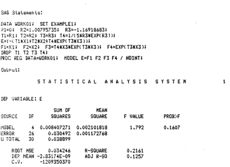
In simple examples such as the proceeding, one can work directly from printed output such as Figure 5a. But anything more complicated requires some programming effort to compute and invert HeH. There are a variety of ways to do this; we shall describe a method that is useful pedagogically as it builds on the ideas of the previous section and is easy to use with a statistical package. It also has the advantage of saving the bother of looking up the critical values of the F distribution.

Suppose that one fits the model

e :II Fl3

+

u

by least squares and tests the hypothesis

H: Hl3 "" h(8) against A: Hl3

*

h(S)

The computed F statistic will be

but since

F :II

[Hl3 - h(;»)'[;(;';)-1;')-1[;; - h(;»)/q

A A N ' A AX

[e - Fl3] [e - Fl3]/(n-p)

....

,

....

we have

At A _lA,A A

o -

(F F) F e -

a

and the computed F statistic reduces to

Thus, any statistical package that can compute a linear regression and test a linear hypothesis becomes a convenient tool for computing the Wald test

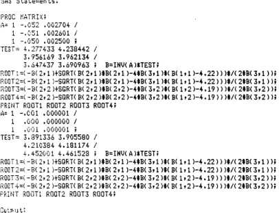
statistic. We illustrate these ideas in the next example.

EXAMPLE 1 (continued). Recalling that the response function is

consider testing

or equivalently

1/5 against