Development of a Time-Resolved Optical Tomography System for Neonatal Brain Imaging

Optical Tomography System for

Neonatal Brain Imaging

Florian E. W . Schm idt, M .Sc.

D epartm ent o f M edical Physics and Bioengineering U niversity College London

Supervisors:

Prof. D avid T. Delpy, FRS Dr. Jerem y C. Hebden

Thesis subm itted for the degree of D octor o f Philosophy (Ph.D.) at the U niversity o f London

All rights reserved

INFORMATION TO ALL USERS

The quality of this reproduction is dependent upon the quality of the copy submitted.

In the unlikely event that the author did not send a complete manuscript and there are missing pages, these will be noted. Also, if material had to be removed,

a note will indicate the deletion.

uest.

ProQuest U642212

Published by ProQuest LLC(2015). Copyright of the Dissertation is held by the Author.

All rights reserved.

This work is protected against unauthorized copying under Title 17, United States Code. Microform Edition © ProQuest LLC.

ProQuest LLC

789 East Eisenhower Parkway P.O. Box 1346

This Ph.D. project involved making a major contribution to the development and evaluation of a prototype medical optical tomography system. The time-resolved 32-channel instru­ ment is presented, and various instrumental aspects and performance issues are discussed. It has been designed primarily as a continuous bedside monitor for obtaining functional images of premature infants’ brains that are at an increased risk of injury due to dysfunction in cerebral oxygenation or baemodynamics. The fully automated device employs 32 source fibres that sequentially deliver near infrared (NIR) pulsed laser radiation of picosecond duration to the tissue. Transit time measurements of very high temporal resolution (-100 ps FWHM) and stability (-5 ps/b drift, and jitter of similar magnitude) are made between these sources and 32 detector optodes also located on the skin surface. Photons transmitted diffusely through the tissue and collected by the optodes are transmitted to four ultra-fast eight-anode MicroChannel Plate Photomultiplier Tube (MCP-PMT) detectors. Thirty-two fully simplex Time-Correlated Single Photon Counting (TCSPC) channels simultaneously record histograms of the photon flight times at rates of up to about 300,000 counts per second per channel. These so-called Temporal Point Spread Functions (TPSFs) represent the raw data for the image reconstruction. Separate maps of the internal absorption and scattering properties can be reconstructed from purely temporal data without recourse to reference or baseline measurements.

First of all I would particularly like to thank my supervisors, Prof. David Delpy and Dr. Jeremy Hebden. Both have been extremely helpful with my initial grant applications, with their continuous guidance and support throughout this project, and patiently proof-reading my transfer and final Ph D. theses.

This research project was very much a team effort and many special thanks go to the other members of this team: Dr. Martin Fry, who has built many of the electronic modules and neatly rewired the system, and Elizabeth Hillman who made huge efforts in turning raw measurement data into meaningful images as well as contributing to all other aspects of the project. I would also like to thank the members of the theoretical imaging group: Dr. Simon Arridge, Dr. Martin Schweiger, Dr. Hamid Dehghani and Ivo Kwee, who have been a constant source of help and advice.

While it is impossible to mention every person who helped me, I would like to thank Dr. Mark Cope, Dr. David Kirkby and Dr. Roger Springett, who frequently gave assistance on electronic, computing-related and other matters, as well as all other members of the Biomedical Optics Research Group.

Many thanks also go to the staff in the Medical Physics mechanical workshop. Bill Raven, Denzil Booth and Stewart Morrison, who machined several parts for MONSTIR and helped me out on several occasions.

I would like to express my gratitude for discussions on medical issues and the prac­ tical aspects of clinical brain imaging systems with UCLH medical staff Prof. John Wyatt and Dr. Judith Meek. I would also like to thank Prof. John Wyatt and Dr. Martina Noone for collaborating on the neonatal post-mortem study that was carried out in our laboratory.

1999 Inter-Institute Workshop on In Vivo Optical Imaging in Bethesda.

1

Introduction

20

1.1 Motivation and objectives 20

1.2 The optical imaging team 22

1.3 Thesis outline 23

2

Basic Anatomy and Physiology of the Human Brain

25

2.1 Anatomy of the head 25

2.2 Major regions of the brain and their functions 28

2.3 The cerebral circulatory system 31

2.4 Structure and pathologies of the neonatal brain 33

3 An Overview over Existing Medical Imaging Techniques

36

3.1 Radiology and Computed Tomography with x-rays 36

3.1.1 Diagnostic Radiology 36

3.1.2 Computed Tomography 37

3.2 Diagnostic Ultrasound 39

3.3 Magnetic Resonance Imaging 41

3.4 Radioisotope Imaging 44

3.4.1 Single Photon Emission Computed Tomography 44

3.4.2 Positron Emission Tomography 45

3.5 Electrical Impedance Tomography 46

4

Fundamentals of Tissue Optics

48

4.1.3 Optical properties of various tissue types 51

4.2 Modelling of photon transport in tissue 56

4.2.1 The Radiative Transfer Equation 57

4.2.2 Deterministic models 58

4.2.3 Stochastic models 62

5 Current State of Near infrared Spectroscopy and Imaging

65

5.1 Types of instrumentation 65

5.1.1 Continuous intensity instruments 66

5.1.2 Intensity-modulated instruments 67

5.1.3 Time-resolved instruments 68

5.2 Non-localised NIR spectroscopy 68

5.3 Localised NIR spectroscopy 70

5.4 Optical imaging 70

5.4.1 Historical background 71

5.4.2 Time-resolved imaging schemes 73

5.4.3 Current imaging systems 78

6

Instrument Design

82

6.1 Design considerations 82

6.1.1 Reasons for choosing a time-resolved system 82

6.1.2 General system requirements 86

6.1.3 Safety aspects 87

6.2 Instrument description 93

6.2.1 Optical assemblies 95

6.2.2 Electronic modules 119

6.2.3 Instrument control and data acquisition hardware and software 129

7 System Performance Evaluation

141

7.1 Data acquisition efficiency 141

7.1.4 Switching speed 149

7.1.5 Summary 149

7.2 Instrument response 150

7.3 Temporal stability 151

7.3.1 System warm-up 153

7.3.2 Temperature fluctuations 154

7.3.3 PSU stability and noise 154

7.3.4 Wiring and grounding 155

7.3.5 Electronic connectors 155

7.3.6 Laser pulsing stability 155

7.3.7 Reference photodiode 155

7.4 Cross talk 155

7.4.1 Detector cross talk 155

7.4.2 Source cross talk 156

7.5 Reflections 158

7.6 Detector aperture 159

7.6.1 Fibre bundle optode 159

7.6.2 VOA 160

7.7 Sample TPSF measurements 163

8

Imaging Experiments

166

8.1 Experimental procedure 166

8.1.1 Temporal calibration 166

8.1.2 Image data acquisition 169

8.1.3 Data pre-processing 169

8.1.4 Image reconstruction 172

8.2 Phantom images 172

8.2.1 Basic cylindrical phantom 172

8.2.2 3D phantom 181

8.3.2 Finger flexor experiment 191

8.4 Preliminary post-mortem neonatal study 193

8.4.1 Introduction 193

8.4.2 Results 194

9

Discussion

196

9.1 Instrument 196

9.1.1 Hardware additions 196

9.1.2 Performance 199

9.2 Image reconstruction and quality 201

9.3 Future imaging studies 203

9.3.1 Phantom studies 204

9.3.2 Clinical studies 205

9.4 Prospects for clinical and commercial utilisation 206

9.5 Conclusion 207

9.6 Publications resulting from this work 208

Appendix A MPE Calculation for Skin

210

Appendix B MONSTIR Technical Drawings

214

Appendix C MIDAS File Format and Code Details

217

C .l File formats 217

C.2 Code structure 219

Appendix D TOAST Image Reconstruction Software

226

Figure 2-1 Skin and underlying subcutaneous tissue. (Reproduced from [Marieb

1991]). 26

Fi gure 2 -2 Skull. (Reproduced from [Marieb 1991]). 27

Figure 2-3 Meninges. (Reproduced from [Marieb 1991]). 28

Figure 2-4 Cerebrospinal Fluid. (Reproduced from [Marieb 1991]). 28 Figure 2 -5 Major Regions of the Brain. (Reproduced from [Marieb 1991]). 29 Figure 2-6 Major Regions of the cerebral hemispheres. (Reproduced from [Marieb

1991]). 30

Figure 2-7 Major cerebral arteries and the circle of Willis. (Reproduced from

[Marieb 1991]). 31

Figure 3-1 X-ray imaging system. (Reproduced from [Webb 1990]). 36 Figure 3-2 X-ray image of an infant with a fracture in the right parietal bone (c.f. Figure 2-2). (Reproduced from the University of Hawaii John A. Bums School of

Medicine website). 37

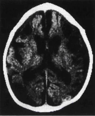
Figure 3 -3 First generation CT scanner. (Reproduced from [Webb 1990]). 38 Figure 3 -4 Computed tomography scan performed at 4 months of age after hypoxic- ischemic cerebral injury at birth. Note the many cysts and enlarged ventricles demonstrating multicystic encephalomalacia (cerebral softening) and cerebral atrophy (shrinkage). The damage is clearly visible because the image was taken four months after the injury occurred. In contrast, a scan taken during, or shortly after, the injury would show very little changes, thus underlining the potential clinical benefits of a new modality such as optical imaging. (Reproduced from [Hill 1996]). 39 Figure 3-5 Parasagittal ultrasound scan demonstrating a large intraventricular haemorrhage forming an echogenic clot adherent to the choroid plexus. (Reproduced

from [Haddad 1991]]). 40

Figure 3 -6 MRI magnetic moment/flux interaction. 41

the area supplied by the MCA (hyposignal), and corresponding haemorrhage (hypersignal) adj acent to the cerebral infarct. (Reproduced from [Haddad 1991]). 42 Figure 3 -8 Functional MRI (fMRI) brain images of the author showing the response to a visual checkerboard stimulus. The low-resolution, thresholded, fMRI image is overlaid onto a standard anatomical image acquired during the same session. From left to right: sagittal, coronal, and transverse sections. (Images acquired with a 2 T Siemens Magnetom system at the Functional Imaging Laboratory, Wellcome

Department of Cognitive Neurology, London.). 43

Figure 3 -9 Transverse SPECT images of the heads of two full-term infants, one normal (left), and the other suffering of cerebral leucomalacia (damage of the white 44 Figure 3-10 PET coincidence detection. (Reproduced from [Webb 1990]). 45 Figure 3-11 Transverse PET scan of the head of a premature infant with intraventricular haemorrhage and haemorrhagic infarct (lack of blood flow leading to tissue damage) in the left cerebral hemisphere. The scale is a linear representation of

Cerebral Blood Flow (CBF). Note the reduction of CBF in 45

Figure 3-12 EIT images of adult visual evoked response, representing impedance changes due to localised increases in blood volume. A total of 31 electrodes were distributed around the head, and 3D images reconstructed into slices assuming the head to be a homogeneous sphere. There are three baseline images followed by a visual stimulus and recovery. The expected area of change is located towards the back of the brain (visual cortex, see inset on bottom right of figure). Images obtained from A. Gibson, T. Tidswell and D. Holder, Department of Clinical

Neurophysiology, UCL [Tidswell 1999]. 47

Figure 4-1 Absorption spectrum of water. 52

Figure 4-2 Absorption spectrum of fat. 5 3

Figure 4-3 Oxygen-haemoglobin dissociation curve. Note that the oxygen saturation of blood leaving the lungs (the arterial saturation) is about 97%, while that of venous blood is still about 67% lower. Hence approximately 30% of the haemoglobin-bound

oxygen is unloaded in the tissues during one cycle through the body. 5 3

Figure 4-4 Absorption spectra of oxy- and deoxyhaemoglobin in the ranges 450-

F igure 4-5 Diagram illustrating the diffuse propagation of light through a thick section of tissue. A narrow input beam of pulsed light is injected and becomes dispersed temporally and spatially through multiple scattering events. The strongly attenuated output pulses are broadened due to the variation in photon flight times. 56 F igure 4-6 A TPSF (right) calculated from a Green’s function for an infinite slab (left). Note that if the finite laser pulse width and detector response is to be taken 60 F igure 5-1 The three fundamental types of NIR spectroscopy/imaging

instrumentation. 66

F igure 5-2 NIRS measurements of Hb and HBO2 concentration changes recorded

during delivery. These reveal changes in the human foetal brain during the transition from foetal to postnatal life. Also note the periodic changes due to uterine contractions. An optode was positioned against the scalp, and the data were recorded using the continuous intensity Hamamatsu NIRO 500 instrument. (Reproduced from

[Peebles 1992]). 69

Figure 5-3 Diagram illustrating two types of time-resolved imaging schemes; (a) isolating shorter flight time photons (usually in an x-y scanning geometry; early

photons 74

Figure 6-1 PMDF computed for an adult head model based on continuous intensity (left) and mean time/phase (right) measurements, respectively. The optode spacing is 4.5 cm, and the data were computed using a finite element implementation of the diffusion approximation to the radiative transfer equation. (Reproduced from [Delpy

1997]). 83

Figure 6-2 Computed TPSFs (top) and their Fourier Transforms (bottom) for a homogeneous, tissue-equivalent, slab of varying thickness in the range 10-50mm. The TPSFs were calculated from a diffusion model based Green’s function as

described in section 4.2.2.1.1. 85

F igure 6-3 Internal structure of the eye. (Reproduced from [Marieb 1991]). 89 F igure 6 -4 MPE expressed in terms of average irradiance versus exposure time (x)

for three different wavelengths. Full-range log scale (top), and detail linear scale

(bottom). 91

F igure 6-5 Schematic diagram of the imaging system. Note that only one source

Figure 6 -6 Photograph of the instrument’s portable main rack, which contains all components apart from the laser source and MCP-PMT chiller unit. Most of the electronics and the control PC are housed at the front of the 19” rack. The VO As and the fibre switch are located on the back, while the MCP-PMT cooling houses can be seen in the top-left part of the side view. The portable cabinet frame is made of

mechanical modular elements supplied by Bosch (Stuttgart, Germany). 95

F igure 6-7 Main optical components of MONSTIR. 96

F igure 6-8 Millennia pump source (back) and Tsunami laser (front) on optical

bench. 96

F igure 6-9 Photograph of the custom-made 19” rack mounted Fibre Switch housing. The optical input and output connectors are located on the left-hand side of the front panel (with the input and only one output fibre connected). The actual DiCon 1x32

switch module is hidden underneath the PCB on the right-hand side. 99

F igure 6-10 Illustration of fibre bundle geometry (left). The packing fraction equals

the shaded area divided by the area of the triangle (right). 100

F igure 6-11 Photograph of a fibre holder ring, which is used for imaging cylindrical phantoms. Thirty-two small-diameter source fibres, and 32 large-diameter detector

fibre bundles are arranged uniformly around its circumference. 101

F igure 6-12 Schematic diagram illustrating the variation in detected intensity (right) for 32 detectors optodes arranged around a circle (left). The large arrow on the left- hand side indicates the source, which in this example is located between detectors 1 and 32. The intensity values are approximations based on a calculation using infinite space Greens functions for all 32 source-detector optode separations (see also section 4.2.2.1). The diameter of the circle in this model is 80 mm, with p / = 1.0 mm"' and Pa

= 0.01 m m ' . 102

F igure 6-13 VOA mask layout. 103

Fi gure 6-14 VO A mask spectral reflectance. 105

F igure 6-15 Illustration of the VOA housing with top plate mounted (left) and

removed (right). (Drawing prepared by Yoko Schmidt). 105

of most VOAs in this picture have been removed, thus revealing the circular VOA masks), and (c) the front panel is mounted on the VOA box, with the 8 detector fibre bundles attached to the individual VOA units. The polymer fibres connecting the VOAs to the MCP-PMT photocathode are mounted at the rear of the VOA box

(hidden). 106

F igure 6-17 Chart of the estimated and measured VOA attenuation values. The measured values for the 8 etched holes (3500 down to 200 |L im ) represent the

averages of all 32 VOAs, and include the standard deviations. Note that differences between the individual channels can be calibrated for should absolute intensity 107

Figure 6-18 Polymer fibre spectral transmittance. 109

Figure 6-19 Picture of the detector assembly. The cylindrical base, which holds the

MCP-PMT, is mounted in a cooling housing (see also Figure 6-6). 109

Figure 6-20 Long-pass filter spectral transmittance. 110

Figure 6-21 (a) General MCP-PMT layout (reproduced from [Knoll 1989]), and (b) radiant sensitivity of various common photocathode materials (reproduced from

[Koyama 1988]). 112

Figure 6-22 Quantum efficiency and radiant sensitivity of a Hamamatsu R4110U-

05MOD MCP-PMT (S/N ET0002; reproduced from Hamamatsu test sheet). 112

F igure 6-23 Waveform of the MCP-PMT (S/N ET0002) recorded at V = -3280 V. Rise time = 205 ps, fall time = 317 ps, width = 390 ps. (Reproduced from Hamamatsu test sheet). See also Figure 6-31 for a density plot of multiple MCP-

PMT output pulses. 113

F igure 6-24 MCP-PMT output pulses and threshold level (left), and typical pulse

height distribution (right). (Reproduced from [Hamamatsu 1995]). 116

F igure 6-25 Count rate and instrument response function width vs. MCP-PMT

supply voltage. 117

F igure 6-26 Scaled diagram of a single MCP-PMT segment with polymer fibre (cj) = 3.0 mm) and illuminated area (({) = 5.5 mm) indicated. Note that approximately 50%

of the photocathode segment is illuminated. 118

F igure 6-27 Photodiode signal recorded with a 1 GHz Tektronix TDS784 digital

oscilloscope. 118

Figure 6-29 Illustration of the constant fraction timing process. 121 F igure 6-30 CFD Monitor output persistence (density) histograms for two different walk settings. The trace shown in (a) has been recorded at a near-optimum walk adjustment voltage of Vw=+2.8 mV, while in (b) the walk is at Vw=-2.9 mV. The trace in the latter is rather distorted and the zero crossing, which is used to generate the logic timing pulses, is not very well defined, as indicated by the arrows. In contrast, trace (a) is typical for a near-optimum adjustment and will result in a

narrower, better shaped, IRF. 122

Figure 6-31 Experimental setup (a), and oscilloscope screenshots (b) of pre­ amplifier output pulse recordings. The PA output is fed through a resistive splitter of very high bandwidth (18 GHz). Pulses with 50% of their original amplitude are fed into the CFD, and the oscilloscope (1 GHz bandwidth TDS784). Traces representing the density of multiple recorded pulse waveforms (persistence histograms) were recorded at two different CFD threshold voltages (Vt = -35 mV and -70 mV). Since the CFD fast NIM logic output is used as the trigger for the oscilloscope, only those pulses whose amplitude is higher than the threshold are recorded. The oscilloscope was set at 200 mV/division. Hence the maximum measured amplitude is —640 mV. However, the recorded signal has been attenuated by the splitter (-6 dB), as well as

the finite bandwidth of the oscilloscope 123

F igure 6-32 PTA timing diagram. 127

F igure 6-33 A PTA time spectrum illustrating the duplication of the recorded curve. 128 Figure 6-34 Schematic diagram indicating the hardware/PC interfacing layout, (i/p: digital input, o/p: digital output, AD: analogue to digital, DA: digital to analogue) 130 F igure 6-35 The four main screens of the MIDAS system control software package. 134 F igure 6-36 Screenshot of the ADF Tool, which is used to automatically create

acquisition protocols. 137

F igure 6-37 Chart of the main MIDAS objects. 140

F igure 7-1 Cooling of the MCP-PMT detector (solid line) and dark count rate (dashed line). The phase delay is thought to be due to the fact that the sensor is

Figure 7-2 Saturation curves of the MCP-PMT (a), PTA (b), and the two combined (c). The dashed lines represent linearity (Rrec=Rtme). The solid lines are the estimates,

and the crosses represent the actual measurements. 146

Figure 7-3 Diagram illustrating the estimated light losses in different components of the MONSTIR detection system. C.f. the system’s main diagram in Figure 6-5. 147 Figure 7-4 Instrument Response Function: linear (a) and logarithmic (b) scales. 150 Figure 7-5 Test illustrating the temporal IRF shift due to physical optode separation. A source fibre and detector fibre bundle were moved apart in discrete steps, and the mean time of the IRF recorded for each position. The measurements agree well with

the calculated delay changes (dashed line). 151

Figure 7-6 Graph illustrating small temporal drift and jitter in 32 channels over a 60

min period. 152

F igure 7-7 Graph showing strong drift and jitter in 32 channels over a 30 min period. Note the different x- and y-axis scales as compared to Figure 7-6. 152 F igure 7 -8 Ambient (room) and MONSTIR temperature (measured above the CFD rack) after start-up at Time = 0. The vertical line on the right-hand side indicates the switching on of the air-conditioning system. If MONSTIR, the MCP-PMT chiller units and the laser system are all switched on, the room temperature can rise up to

about 31°C - despite air-conditioning. 153

F igure 7-9 Cross talk between adjacent channels of an 8-channel MCP-PMT

detector. 156

F igure 7-10 Schematic diagram and measured TPSF illustrating the pre-peak due to

cross talk between the source chaimels. 157

F igure 7-11 Diagram illustrating the interfaces at which reflections occur. 158 F igure 7-12 Chart illustrating the dependence of the mean time on the source- detector optode separation (b). The mean times were calculated using an analytical (Green’s function) model of a homogeneous slab in reflectance geometry (a). 160 F igure 7-13 Instrument responses recorded for two VOA settings, where a source fibre was placed into direct contact with the detector fibre bundle. VOA Position 8 162 F igure 7-14 Two nearly identical TPSFs recorded on a tissue equivalent phantom at the two extreme VOA settings. The little spike near the top of the curves is

Figure 7-15 The mean time recorded on a tissue-equivalent phantom for all eight VOA settings (holes). The data points are average values with their corresponding

standard deviations obtained from ten successive measurements, 163

Figure 7-16 Mean time curves for 22 detector channels recorded with MONSTIR

compared to FEM and Monte Carlo model simulations. 164

Figure 7-17 Measured (MONSTIR) and simulated (Monte Carlo) TPSFs corresponding to source no. 1 and detector no, 6 (a). The measured curve is scaled to its maximum value, while the Monte Carlo curve, because it is rather noisy, is scaled to the maximum of a Green’s function curve fit (not shown). The Monte Carlo curve convolved with an instrument response function is shown in (b), giving a much

improved agreement with the measured data. 165

Figure 8-1 Source calibration: all 32 source fibres are arranged around the circumference of a clear cylinder and illuminated sequentially. Note that for clarity

not all fibres are shown in this illustration. 167

Figure 8 -2 Detector calibration: all 32 detector fibre bundles are illuminated

simultaneously by a source at the centre. 168

F igure 8-3 Absolute calibration: a source fibre and detector fibre bundle are placed

at a known separation from each other. 168

F igure 8-4 Plot illustrating the integrated intensity, mean time and variance of a

TPSF. 170

F igure 8-5 Diagram of the phantom indicating the three embedded cylinders and the

fibre holder ring. 173

F igure 8-6 Photograph of the basic cylindrical phantom (c.f. illustration in Figure 8 - 5). A source fibre can be seen on the left, and 8 detector fibre bundles on the right. 174 F igure 8-7 A cross-section of the phantom indicating the three regions of interest (a), and the absorption (b) and scattering (c) profiles corresponding to iteration 30 of

the image reconstruction process. 174

F igure 8-8 Photograph of the solid tissue-equivalent phantom with the fibre holder ring and all 2x32 fibres mounted. Note the small-diameter source fibres, which are

F igure 8-9 TPSFs (b) recorded by the 22 active detectors opposite source no 1 (a). Each TPSF consists of up to -10*^ photons, and the curves are normalised to their

respective maximum values. 176

F igure 8-10 The three commonly used data types, mean time (a), variance (b) and Laplace transform (c) extracted from the TPSF curves presented in Figure 8-9 (b). 178 F igure 8-11 The reconstructed absorption and scattering profiles corresponding to 35 iterations are shown in (a) and (b) respectively. The greylevels are scaled

globally. 180

F igure 8-12 Absorption (b) and scattering (c) profiles of the phantom depicted in

(a). 181

Figure 8-13 Cross-section of the 3D phantom (a) and side view (b). 182

Figure 8-14 Photograph of the 3D phantom showing the fibre assembly in one of the

14 acquisition planes. 183

F igure 8-15 Reconstructed absorption and scattering profiles for 14 different

transverse planes along the axis of the 3D phantom. 184

F igure 8-16 Transverse (a) and vertical (b) cross-sections of the absorbing cylinder C, which is centred at 100 mm above the base. The vertical cross-section consists of

one data point per slice. 185

Figure 8-17 Transverse (a) and vertical (b) cross-sections of the scattering cylinder

A, which is centred at 50 mm above the base. 186

Figure 8-18 Cross-section of the differential absorption phantom (a), and

reconstructed absorption difference image (b). 187

Figure 8-19 Three absorption profiles as linear cross-sections through cylinders A,

Bi & B2 and Ci & C2. 188

Figure 8-20 Illustration of the human forearm’s cross-section (a). Muscle groups, bones and some of the blood vessels (a) (based on a diagram from [Marieb 1991]). An MRI scan of the subject’s forearm (b), while inserted into the fibre holder ring, was acquired at the Middlesex Hospital with the assistance of Dr. Sean Smart. 189 F igure 8-21 Photograph of the subject’s arm. The fibre holder ring is positioned

reproducible position, while the handle on the left is a strain gauge used in finger

flexor experiments. 189

F igure 8-22 Absorption and scattering images of the forearm acquired at 790 nm and 820 nm. They are reproduced using a colour scale in order to better represent the

subtle variations in the absorption maps. 191

F igure 8-23 Absorption difference image representing the alteration in absorption at

820 nm between the rest and active states of the forearm. 192

F igure 8-24 Photograph of the deceased infant’s head. The fibre assembly is arranged around the circumference, channel no. 25 being at the top (c.f. Figure 8-25

(a), which has the same orientation). 193

F igure 8-25 Map of the source and detector optode positions (a), which were determined using graph paper held against the fibre assembly after the head was withdrawn at the end of the experiment. The outline represents a top view of the transverse section indicated by the fibre assembly in the photograph in Figure 8-24. Sample TPSFs recorded at 820 nm by detector no. 7 corresponding to three different

sources (1, 29 and 19) are shown in (b). 195

Figure 9-1 Photograph of the IMRA Femtolite 780 nm fibre laser head during

evaluation in our laboratory. 198

F igure 9 -2 Photograph of the 3D phantom and three rings holding the source and detector optodes in a cross-planar arrangement (a). The bottom ring contains all 32 source fibres, while the two upper rings each hold 16 detector fibres. Data were acquired for three similar arrangements (sources on bottom, middle and top). A tissue-equivalent phantom that resembles a premature infant’s head is shown in (b). 204 Figure A -1 Plot of exposure time (î) versus laser repetition frequency (flaser) for

three different pulse durations. 213

F igure B -1 Technical drawing of the VOA housing. 215

Figure B -2 Technical drawing of the MCP-PMT fibre and long-pass filter holder. 216 Figure D -1 A sample 2D FEM mesh consisting of 7392 triangular elements. 227

List of Tables

Table 4-1 Optical properties of various tissue types. 55

Table 6-1 Millennia pump laser specification. 97

Table 6 -2 Tsunami picosecond laser specifications. 98

Table 6-3 DiCon fibre switch specifications. 98

Table 6 -4 Summary of VGA features. 108

Table 6 -5 Hamamatsu MCP-PMT specifications (averages or ranges of all MCP-

PMTs, where appropriate). 114

Table 6 -6 Pre-amplifier specifications. 120

Table 6 -7 CFD specifications. 124

Table 6 -8 Amplifier/Timing Discriminator specifications. 124

Table 6 -9 Delay unit specifications. 125

Table 6-10 F ast fan-out unit specifications. 125

Table 6-11 PTA specifications. 126

Table 6-12 HV PSU specifications. 129

Table 6-13 Digital 10 card specifications. 131

Table 6-14 Multifunction 10 card specifications. 132

Table 6-15 VOA stepper motor controller specifications. 132

Table 7-1 Sununary of estimated detection loss factors in the individual components of the MONSTIR detection system. The combined losses for each component can be looked up in Figure 7-3. Note that these are only very approximate values. Most are derived from manufacturer's data sheets, and have been experimentally verified where possible. However some values are rough estimates and are marked as such. 149

1 Introduction

The field known as biomedical optics has evolved considerably over the last couple of decades. The widespread availability of suitable laser sources and detectors has aided the rapid development of new optical technologies for the monitoring and diagnosis, as well as treatment, of patients. Furthermore, new optical techniques are helping to advance fundamental biomedical research. My Ph.D. project involved undertaking a leading role in the development and evaluation of a prototype multi-channel time-resolved optical tomographic imaging system, whose principal application is the monitoring of premature infants’ brains.

1.1

Motivation and objectives

Premature babies have an increased risk of cerebral haemorrhage, and both the preterm and the full term infant can suffer from blood fiow or oxygen deficiencies (hypoxic-ischemia) leading to severe neurodevelopmental disorders. There is currently no device capable of

continuously monitoring regional variations in cerebral blood volume and oxygenation at

the cotside. Hence research at University College London (UCL) has focussed on the development of a portable instrument that employs near infrared (NIR) laser light for imaging the neonatal brain, and which is capable of detecting brain pathologies as well as monitoring response to treatment.

functional images and quantify changes in cerebral blood volume or oxygenation, thereby revealing important physiological information before irreversible structural damage occurs. In comparing the proposed new modality with established techniques, it can be argued that although diagnostic ultrasound imaging or x-ray Computed Tomography (CT) are effective at detecting haemorrhages, they cannot visualise oxygenation. Blood-Oxygenation Level Dependent (BOLD) Magnetic Resonance Imaging (MRI), while providing oxygenation- sensitive data, is difficult to perform on neonates because they require transportation to the radiology unit, sedation if they are not asleep, and must be stripped of all metal-containing probes. Because of these complications, and its high cost, MRI can only provide an occasional snapshot in response to a suspected condition, rather than a permanent bedside monitor. Similarly, Single Photon Emission Computed Tomography (SPECT) and Positron Emission Tomography (PET), while providing useful functional information, do not allow continuous bedside monitoring. Moreover, because they require the injection of radioactive substances, SPECT and PET are invasive and not free from risk. In fact, their use on neonates is restricted in many countries, including the USA and UK.

be very useful clinically, especially if they can be acquired continuously, with the patient lying relatively undisturbed in an incubator in a neonatal intensive care environment.

It was the objective of my Ph.D. project to make a major contribution to the devel­ opment of such a multi-channel time-resolved neonatal brain imaging system. The work involved completing its construction, evaluating the instrument performance, and conduct­ ing phantom and preliminary clinical imaging studies.

1.2

The optical imaging team

This research project was carried out in the Biomedical Optics Research Group (BORG), which is located within the Department of Medical Physics & Bioengineering at UCL. The research interests of BORG primarily concern the development of new optical monitoring instruments and techniques for biomedical applications. Within BORG, optical tomographic imaging represents one of the main research activities, and there are two closely collabo­ rating groups, one focussing on theory, and the other on the experimental side:

Head of BORG Prof. David Delpy, FRS

Experimental Imaging Group Dr. Jeremy Hebden Dr. Martin Fry Elizabeth Hillman Florian Schmidt

Theoretical Imaging Group Dr. Simon Arridge Dr. Martin Schweiger Dr. Hamid Dehghani Ivo Kwee

The experimental group is based at the Department of Medical Physics & Bioengineering, while the theoretical group is also partly based at the Department of Computer Science. My Ph D. supervisors were Prof. David Delpy and Dr. Jem Hebden. Inevitably, given the scale and complexity of this research project, the development of the imaging system was in every aspect a team-effort that involved all group members. Everyone contributed in some way to most aspects of the work.

where appropriate, construction, of most optical and electronic components (e.g. fibre assemblies) or sub-systems (e.g. fibre switch). I designed the Variable Optical Attenuators (VOAs), constructed their mechanical, electrical and optical parts, and developed the corresponding computer code. The VOA controller was custom-made according to my specifications. The overall system is fully computer controlled, and I built or integrated much of the interfacing hardware. An extensive instrument control and data acquisition software package was developed entirely by myself. But perhaps most importantly, I played a leading part in the overall instrument design and system integration, i.e. in putting the individual components together and making them function as a whole system. Following completion of the prototype, I made extensive efforts to optimise and evaluate the system’s performance, and conducted phantom and adult arm imaging experiments as well as a preliminary post-mortem neonatal study.

1.3

Thesis outline

In writing this thesis I have attempted to provide a thorough background of the medical, physical and technological aspects of NIR tomographic brain imaging. A large section of the thesis is devoted to an in-depth discussion of the system’s design features and perform­ ance characteristics. Finally, the experimental procedures and results from initial imaging tests are described. Although neonatal brain images have not been obtained yet, the design and performance characteristics of the system were optimised with that application in mind. Chapter 2 contains a description of the anatomy and physiology of the human head in general, and concludes with a section focusing on the neonatal brain and common neuro­ logical conditions. The aim of this chapter is to present some relevant medical background which will underline the motivation, challenges and design considerations related to the development of this type of imaging modality.

Chapter 3 provides brief descriptions of the established medical imaging modalities. Sample images of neonatal brains are included where possible in order to aid comparison between these modalities and optical imaging.

Chapter 4 contains a general introduction to the physics and mathematics of light propaga­ tion through biological tissue. An understanding of these principles provides the foundation of any image reconstruction scheme.

Chapter 6, which is by far the most extensive, begins with a discussion of the system design considerations. A brief account of the functioning of the instrument as a whole is then followed by a detailed description of the individual optical and electronic assemblies, as well as the control software. In addition to sununarising a major part of my Ph.D. project, this chapter also serves to document relevant technical details.

While chapter 6 focuses on individual components, the performance of the fully integrated system is analysed in chapter 7. A considerable amount of time was spent tackling unprecedented technological problems, and the understanding, evaluation and optimisation of the system characteristics formed an integral part of this research project.

Chapter 8, the final results chapter, describes the principal imaging tests performed with this instrument to date. An outline of the experimental procedures is followed by a presentation of initial studies on phantoms that mimic the premature neonatal brain in both size and optical properties. Recently acquired scans of an adult forearm represent the first ‘clinicar images obtained with the prototype instrument, and the description of a prelimi­ nary non-imaging neonatal study concludes the chapter.

Finally, chapter 9 provides a discussion of the work done so far and the prospects for the future of this project and medical optical tomography in general.

2 Basic Anatomy and Physiology of the

Human Brain

This chapter contains some basic background on the anatomy and physiology of the human brain relevant to this project. The final section focuses on the neonatal brain and some common pathologies.

2.1

Anatomy of the head

The human nervous system consists of the central nervous system (CNS) and peripheral

nervous system (PNS). The former consists of the brain and spinal cord, while the latter

composes the nerves extending to and from the brain and spinal cord. The primary functions of the nervous system are to monitor, integrate (process) and respond to informa­ tion inside and outside the body. The brain consists of soft, delicate, non-replaceable neural tissue. It is supported and protected by the surrounding skin, skull, meninges and cerebro­ spinal fluid.

Skin

The skin constitutes a protective barrier against physical damage of underlying tissues, invasion of hazardous chemical and bacterial substances and, through the activity of its sweat glands and blood vessels, it helps to maintain the body at a constant temperature. Together with the sweat and oil glands, hairs and nails it forms a set of organs called the

integumentary system. Figure 2-1 shows a cross-section of the skin and underlying

subcutaneous tissue. The skin consists of an outer, protective layer, the epidermis and an inner layer, the dermis. While the top layer of the epidermis, the stratum comeum, consists of dead cells, the dermis is composed of vascularised fibrous connective tissue. The

subcutaneous tissue, located underneath the skin, is primarily composed of adipose tissue

Hair sh a ft M eissn er's

c o rp u sc le Stratu m co m e u m

S tratu m lucldum D erm al pap illae

Stratu m gran u lo su m F re e n e rv e

Stratu m sp in o su m end in g

Stratu m b a s a le (oil) g lan d

S e n s o ry n e rv e fiber

Papillary lay er

R eticular layer A rrector

pill m u scle

Hair follicle

Hair root

Epiderm is

P a c in ia n co rp u sc le

_ H yp od erm is (superficial fasc ia)

Eccrin e s w e a t g lan d

A d ip o se tis s u e R oot hair plexus

Figure 2-1 Skin and underlying subcutaneous tissue. (Reproduced from [Marieb 1991]).

Skull

Depending on their shape, bones are classified as long, short, flat or irregular. Bones of different types contain different proportions of the two types of osseous tissue: compact and spongy bone. While the former has a smooth structure, the latter is composed of small needle-like or flat pieces of bone called trabeculae, which form a network filled with red or yellow bone marrow. Most skull bones are flat and consist of two parallel compact bone surfaces, with a layer of spongy bone sandwiched between. The spongy bone layer of flat bones (the diploë) predominantly contains red bone marrow and hence has a high concen­ tration of blood. The skull is a highly complex structure consisting of 22 bones altogether. These can be divided into two sets, the cranial bones (or cranium) and the facial bones.

While the latter form the framework of the face, the cranial bones form the cranial cavity

that encloses and protects the brain. All bones of the adult skull are firmly connected by

sutures. Figure 2-2 shows the most important bones of the skull. The frontal bone forms the

magnum, which is a large hole allowing the inferior part of the brain to connect to the spinal cord. The remaining bones of the cranium are the temporal, sphenoid and ethmoid bones.

C o ro n al su tu re

P arietal b o n e

Frontal b o n e

S p h e n o id b o n e

E thm oid b o n e T em poral b o n e

L acrim al b o n e

L a m b d o id a l Lacrim al f o s s a

s u tu re

N a sa l b o n e

Z y g o m a tic b o n e

Maxilla

M astoid p r o c e s s S qu am o sal sutu re

O c c ip ita l b o n e

Z y g o m a tic p r o c e s s

O c c ip ito m a s to id su tu re

E x tern al au d ito ry m e a tu s

Styloid p r o c e s s

M an d ib u lar c o n d y le

M an d ib u lar n o tch

M an d ib u lar ram u s

M an d ib u lar a n g le C o ro n o ld p r o c e s s

Alveolar m arg in s

M an d ib le

M ental fo ra m en

Figure 2-2 Skull. (Reproduced from [Marieb 1991]).

Meninges

The meninges (Figure 2-3) are three connective tissue membranes enclosing the brain and

the spinal cord. Their functions are to protect the CNS and blood vessels, enclose the

venous sinuses, retain the cerebrospinal fluid, and form partitions within the skull. The

outermost meninx is the dura mater, which encloses the arachnoid mater and the innermost

pia mater.

Cerebrospinal fluid

Cerebrospinal flu id (CSF) is a watery liquid similar in composition to blood plasma. It is

formed in the choroid plexuses and circulates through the ventricles into the subarachnoid

space, where it is returned to the durai venous sinuses by the arachnoid villi. The prime

Superior sagittal sinus Subdural space Subarachnoid space

Skin of scalp

Periosteum

- Bone of skull

Periosteal Meningeal

Arac _Dura

mater

in o id membrane Pia mater

A rachnoid villus

Blood vessel

Falx cerebri (in longitudinal fissure only)

Figure 2-3 Meninges. (Reproduced from [Marieb 1991]).

Superior sagittal sinus Superior cerebral vein Ctioroid Plexus Cerebrum covered witti pia m ater Septum pellucidum C o rpus callosum Inlerventricular foram en Third ventricle

P itu ita r y g l a n d

Cerebral aq u ed u ct l ateral aperture Fourth ventricle M edian aperture

S u b arach n o id s p a c e Arachnoid M eningeal d ura m ater Periosteal d ura m ater Great cerebral vein Tentorium cerebelli Straight sinus C onfluence of sin u ses Cerebellum

Choroid Plexus Cerebral v e sse ls that supply choroid plexus

Central c a n al of spinal cord Spinal du ra m ater (durai sh e ath )

Inferior e n d of spinal co rd

Filum term inale (inferior en d of pia m ater)

Figure 2 -4 Cerebrospinal Fluid. (Reproduced from [Marieb 1991]).

2.2

Major regions of the brain and their functions

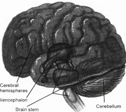
The major regions of the brain (Figure 2-5) are the cerebral hemispheres, diencephalon,

C ere bra l h e m isp h e re s

D ience pha lo n

B rain stem C e re b e llu m

Figure 2-5 Major Regions of the Brain. (Reproduced from [Marieb 1991]).

Cerebral hemispheres

The cerebral hemispheres (Figure 2-6), located on the most superior part of the brain, are

separated by the longitudinal fissure. They make up approximately 83% of total brain mass, and are collectively referred to as the cerebrum. The cerebral cortex constitutes a 2-4 mm thick grey matter surface layer and, because of its many convolutions, accounts for about 40% of total brain mass. It is responsible for conscious behaviour and contains three different functional areas: the motor areas, sensory areas and association areas. Located internally are the white matter, responsible for communication between cerebral areas and between the cerebral cortex and lower regions of the CNS, as well as the basal nuclei (or

basal ganglia), involved in controlling muscular movement.

Diencephalon

The diencephalon is located centrally within the forebrain. It consists of the thalamus,

hypothalamus and epithalamus, which together enclose the third ventricle. The thalamus

acts as a grouping and relay station for sensory inputs ascending to the sensory cortex and association areas. It also mediates motor activities, cortical arousal and memories. The hypothalamus, by controlling the autonomic (involuntary) nervous system, is responsible for maintaining the body’s homeostatic balance. Moreover it forms a part of the limbic

system, the ‘emotional’ brain. The epithalamus consists of the pineal gland and the CSF-

Superior

C ereb ral cortex

C ereb ral white m atter

nsula Lateral su eu s B asal nuclei

Interior

Longitudinal fissure S e p tu m pellucidum C o rp u s callosum Anterior horn of lateral ventricle

C a u d a te n u cleu s P u t a m e n l ^ G lobus h Lentiform v pallidus _| n ucleu s T halam us of d ie n c e p h a lo n Interior horn of laleral ventricle Third ventricle

Figure 2 -6 Major Regions of the cerebral hemispheres. (Reproduced from [Marieb 1991]).

Brain stem

The brain stem is similarly structured as the spinal cord: it consists of grey matter sur­ rounded by white matter fibre tracts. Its major regions are the midbrain, pons and medulla

oblongata. The midbrain, which surrounds the cerebral aqueduct, provides fibre pathways

between higher and lower brain centres, contains visual and auditory reflex and subcortical motor centres. The pons is mainly a conduction region, but its nuclei also contribute to the regulation of respiration and cranial nerves. The medulla oblongata takes an important role as an autonomic reflex centre involved in maintaining body homeostasis. In particular, nuclei in the medulla regulate respiratory rhythm, heart rate, blood pressure and several cranial nerves. Moreover, it provides conduction pathways between the inferior spinal cord and higher brain centres.

Cerebellum

The cerebellum, which is located dorsal to the pons and medulla, accounts for about 11% of

2.3

The cerebral circulatory system

Blood is transported through the body via a continuous system of blood vessels. Arteries

carry oxygenated blood away from the heart into capillaries supplying tissue cells. Veins

collect the blood from the capillary bed and carry it back to the heart. The main purpose of blood flow through body tissues is to deliver oxygen and nutrients to and waste from the cells, exchange gas in the lungs, absorb nutrients from the digestive tract, and help forming urine in the kidneys. All the circulation besides the heart and the pulmonary circulation is called the systemic circulation.

Since it is the ultimate aim of this research project to image cerebral oxygenation and haemodynamics some aspects of the cerebral circulatory system are described below.

A nterior

F r o n ta l lo b e

C ircle O f W illis:

• A n te rio r c e r e b r a l a r t e r y • A n te rio r

c o m m u n i c a t in g a r te r y

• P o s te r io r c o m m u n i c a t in g a r te r y

• P o s te r io r c e r e b r a l a r te r y

B a s ila r a r t e r y

V e r te b r a l a r te r y

O c c i p it a l ---3 ^ ---C e r e b e l l u m lo b e

Posterior

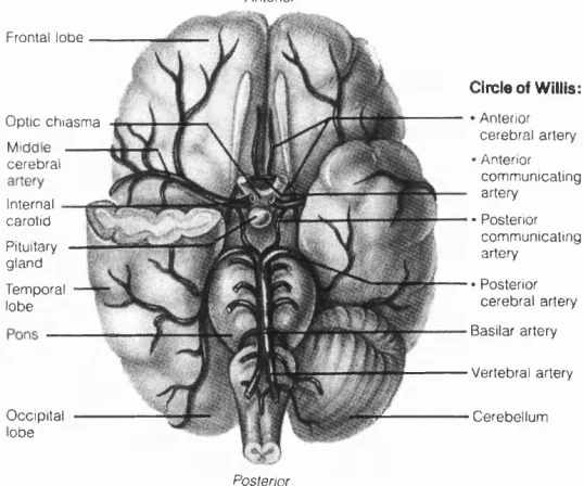
Figure 2-7 Major cerebral arteries and the circle of Willis. (Re­ produced from [Marieb 1991]).

o p t i c c h i a s m a M id d e c e r e b r a l

In te rn a l c a r o t id P itu ita ry g l a n d T e m p o ra l lo b e

Blood supply to the brain

Figure 2-7 shows an overview of the arterial system supplying the brain. The major arteries are the vertebral and internal carotid arteries. The two posterior and single anterior

communicating arteries form the circle o f Willis, which equalises blood pressures in the

on the brain’s surface. Hence occlusion of these arteries usually results in localised tissue damage.

Cerebral haemodynamics

The cardiac output is about 5 1/min of blood for a resting adult. Blood flow to the brain is about 14% of this, or 700 ml/min. For any part of the body, the blood flow can be calcu­ lated using the simple formula

Blood flow = (2.1)

Resistance

Pressure in the arteries is generated by the heart which pumps blood from its left ventricle into the aorta. (Since pressure was historically measured with a mercury manometer, the units are commonly expressed in terms of [mm Hg], although the official SI unit is the Pascal [Pa].) Resistance arises from friction, and is proportional to the following expression

r, . * Vessel Length

Resistance Viscosity x ----— ^ (2 2)

(Vessel Diameter)"* ^

Hence blood flow is slowest in the small vessels of the capillary bed, thus allowing time for the exchange of nutrients and oxygen to surrounding tissue by diffusion through the capillary walls.

Approximately 75% of total blood volume is ‘stored’ in the veins which, because of their high capacity, act as reservoirs. Their walls distend and contract in response to the amount of blood available in the circulation. However, the function of cerebral veins, formed from sinuses in the dura mater, is somewhat different from other veins of the body, as they are non-collapsible.

Autoregulation

change their diameter about 4-fold, corresponding to a 256-fold change in blood flow. Only when the brain is very active is there an exception to the close matching of blood flow to metabolism, which can rise by up to 30-50% in the affected areas. It is an aim of PET, functional MRI, near infrared spectroscopy (NIRS), and, possibly, near infrared imaging, to detect or image such localised changes in cortical activity and associated blood flow.

2.4

Structure and pathologies of the neonatal brain

Having introduced some basics of the anatomy and physiology of the adult brain, this section focuses on the specific differences in the neonate, as well as common neonatal pathologies which have motivated the construction of an instrument capable of imaging cerebral oxygenation, blood volume and, possibly, myelination.

The embryonic brain and spinal cord develop from the neural tube, which is formed by the fourth week of pregnancy. The brain grows immensely in both size and complexity during pregnancy and even soon after birth. Because a membranous skull restricts expan­ sion, the forebrain is bent towards the brain stem, and the cerebral hemispheres almost completely envelop the diencephalon and midbrain. Moreover, the spatial restrictions cause the cerebral hemispheres to increase their surface area by becoming highly convoluted such that about two thirds of its surface are hidden in its folds. The skull bones of the foetus and neonate are soft and the sutures are not yet fused. Hence the skull is very flexible and deforms under light pressure. Brain development of the foetus, neonate and infant are more thoroughly reviewed by [Herschkowitz 1988].

Compared to the adult, neonates have a smaller head size (ca. 6-12 cm in diameter), thinner surface tissue, skull and CSF layers, lower scattering coefficients of grey and white matter (due to lesser myelination in the case of white matter), as well as a comparatively small mismatch between the two (see also Table 4—1). These anatomical features are all favourable to NIR imaging. The neonatal skull, because it is less mineralised, may also have a lower scattering coefficient, but there is no data at present. All these factors greatly benefit penetration of light deep into the white matter and enable measurements to be made across the head, which is essential for tomographic imaging.

bloodstream. A higher oxygen affinity of neonatal haemoglobin (dissociation curve shifted to the ‘left’, c.f. Figure 4—3) compensates for this. Over a period of about 6 months after delivery the neonatal haemoglobin is gradually substituted by the adult haemoglobin, which has a lower oxygen affinity.

The autoregulation mechanism of the (adult) brain was discussed in the previous section. However, in the newborn infant, and particularly in the very preterm infant, there is no consensus on whether, or to what extent, autoregulation in the brain occurs. It is also not clear what effect ischaemia has on cerebral blood flow and the evolution of haemorrhage.

Neurodevelopmental disorders in some preterm infants are due to either hypoxic- ischaemic damage to the periventricular white matter, or to intraventricular haemorrhage and its consequences. The period of highest risk is between 26 and 32 weeks of gestation. In preterm infants the majority of haemorrhages occur into the ventricles and the surround­ ing white matter, the periventricular region. Hypoxic-ischaemic damage is caused by cerebral underperfusion, often combined with a global oxygen deficiency due to an impaired lung function. It also affects the periventricular white matter, which is thought to be a result of the following two effects:

• Increased vulnerability due to high metabolic demands at this phase of the brain development.

• The area is at a ‘watershed’ of perfusion from the territories of the posterior and middle cerebral arteries (c.f. Figure 2-7).

Enduring neurodevelopmental disorders can lead to diminished neurological function in later life, and in particular spasticity, since motor fibres run through this region of the white matter. Given the potential of the premature infant’s developing brain to repair some damage, spasticity is often restricted to stiff limbs and/or subtle learning disabilities.

Cerebral damage in the mature infant is most commonly a result of perinatal ( ‘birth’) asphyxia, leading initially to cerebral oedema (resulting in compressed ventricles and flattening of the convolutions of the brain), and later to tissue necrosis (tissue death) and apoptosis (cell suicide). The subcortical white matter, basal ganglia, cerebellum and brainstem are the areas predominantly affected, frequently leading to learning disabilities or global developmental delay and cerebral palsy.

3 An Overview over Existing Medical

imaging Techniques

This chapter introduces the most important clinically established medical imaging modali­ ties, A more thorough treatment on the subject can be found in [Webb 1990] or [Curry 1990],

3.1

Radiology and Computed Tomography with x-rays

3.1.1 Diagnostic Radiology

X-rays were discovered by W. C. Rontgen in 1895 and the prospect for medical diagnosis was immediately recognised [Classer 1934], They penetrate most biological tissues with little attenuation, and thus provide a com­

paratively simple means to produce shadow, or projection, images of the human body. The radiographic image represents the distribution of x-ray photons transmitted through the patient. Hence it is a 2D projection of the attenuating properties of tissues along the path of the detected x-rays. The principal interactions causing attenuation are photoe­ lectric absorption and (inelastic) scattering.

Figure 3-1 illustrates a simplified x- ray imaging system. Photons are either scattered, absorbed or transmitted without interaction. Most scattered photons are

X-ray tube

Patient

£7 o D o/o o irn d\p D a a 0 a«3 aQ Anti-scatter grid

13. A lÊ Receptor

removed by an anti-scatter device (e.g. a lead grid). The detector is either a screen-fiim system, an x-ray photographic film or an image intensifier. Commonly used photon energies range from 17-150 keV, the choice for a particular application or tissue probed being a trade-off between acceptable radiation dose and achievable image contrast. Bones cause significantly higher attenuation than soft tissues, as their photoelectric cross-section and density is higher. The resulting higher contrast means that x-ray diagnostic radiology is particularly suitable for imaging (broken) bones as is demonstrated in the example in Figure 3-2.

mm

Figure 3-2 X-ray image of an infant with a fracture in the right parietal bone (c.f. Figure 2-2). (Reproduced from the University of Hawaii John A. Bums School of Medicine website).

3.1.2 Computed Tomography

Conventional radiography provides no depth information, as the 3D body structure is projected onto a 2D image. Another limitation is the low soft tissue contrast, which is particularly important in brain imaging, where the soft tissues are enclosed by the highly attenuating skull. In contrast, x-ray computed tomography (CT) imaging produces thin 2D sections of the body, approximately 1 mm in thickness. Sub-millimetre spatial resolution with good discrimination between tissues (better than 1% attenuation change) can be achieved.

In 1972 G. N. Hounsfield first presented a clinical CT scanner at the Annual Con­ gress of the British Institute of Radiology, the design of which is described in [Hounsfield

the discovery of x-rays. First generation CT systems employed a narrow pencil beam from a collimated source that scans linearly across the patient in order to obtain a parallel projection. The system is then rotated to obtain several such projections. Figure 3-3 shows a schematic setup.

60th scan

X-Ray tube

Detector \

Figure 3-3 First generation CT scanner. (Reproduced from [Webb 1990]).

The data acquisition time was about 4 minutes. Since its development in the early 1970s, several generations have been developed and marketed. Current fourth generation CT scanners have a much faster scan speed of about 4-5 seconds. This allows the acquisition of scans with very little motion blur, since the patient can be asked to stop breathing during this period. A rotating fan beam x-ray source with a continuous ring of about 1000 detectors makes this possible. There are now fifth generation systems available with scan times of only a few milliseconds, thus allowing effective ‘real-time’ imaging.

Tomographic slice images representing attenuation values are reconstructed by inverting the measured projection data. The underlying mathematical principles were originally developed by J. Radon in 1917 ([Radon 1917]), long before the first prototypes were constructed. The method most commonly used today is called filtered backprojection and employs the following steps.

1. Record projections at different angles around the object to be imaged.

2. Convolve each projection with a filter function (which prevents the occurrence of the ‘star artefact’ in conventional backprojection).

The underlying mathematics, as well as other reconstruction schemes, are described in more detail elsewhere [Webb 1990]. A sample CT scan of a term baby suffering from hypoxic- ischaemic cerebral injury at birth is shown in Figure 3-4.

Figure 3 -4 Computed tomography scan performed at 4 months of age after hypoxic- ischemic cerebral injury at birth. Note the many cysts and enlarged ventricles (dark regions) demonstrating multicystic encephalomalacia (cerebral softening) and cere­ bral atrophy (shrinkage). The damage is clearly visible because the image was taken four months after the injury occurred. In contrast, a scan taken during, or shortly after, the injury would show very little changes, thus underlining the potential clinical bene­ fits of a new modality such as optical imaging. (Reproduced from [Hill 1996]).

3.2

Diagnostic Uitrasound

In diagnostic ultrasound imaging, high frequency pulses of acoustic energy are emitted into the patients’ body where they experience reflection at boundaries between tissues of different characteristic impedance. From the measurement of time delay and intensity of the reflected pulses (echoes), an image indicating tissue interfaces can be reconstructed. Ultrasound imaging is considered to involve negligible risk, provided that the incident intensities are sufficiently small. The relatively simple technology employed makes it also rather inexpensive as compared to other clinical imaging modalities.

c = (3.1)

where K is the bulk elastic modulus and po the tissue density. The average speed of sound in soft tissues is 1540 m/sec, with variations of about ±6%. These are mainly due to changes in elasticity, rather than density, and are usually ignored in the reconstruction of images. As most biological tissues are effectively fluids, ultrasound waves are always longitudinal. The

characteristic acoustic impedance, Z, of tissue is defined as

^ ~ “ V (3. 2)

Hence, in analogy to Fresnel’s formula in optics, the intensity of a sound beam reflected at a normal boundary between media with acoustic impedances Zy and Z2, relative to the

incident intensity, is given by

R = ^ 2 ~ ^ i

Z2 + Z| (3.3)

Figure 3-5 Parasagittal ultrasound scan demonstrating a large intraventricular haemorrhage forming an echogenic clot adherent to the choroid plexus. (Repro­ duced from [Haddad 1991]]).