Choice of Priors and Variable Selection in Bayesian Regression

(1)

Choice of Priors and Variable Selection in Bayesian Regression

Olusanya .E. Olubusoye (Department of Statistics, University of Ibadan, Nigeria)

Onyeka C. Okonkwo (Department of Statistics, University of

Ibadan, Nigeria)

(2)

354

Author (s)

Olusanya E. Olubusoye Department of Statistics,

University of Ibadan, Nigeria E-mail:[email protected],

Onyeka C. Okonkwo Department of Statistics,

University of Ibadan, Nigeria

E-mail:[email protected]

Choice of Priors and Variable Selection in Bayesian Regression

Abstract

This study is focused on the applications of the Bayes theory to Normal linear Regression model in choosing prior distributions for the parameters of interest and in the selection of variables for inclusion/deletion from a model-in the case of a reduced model. For the choice of prior distribution for the regression parameters β, two choices of priors were employed, these are: (i) the Non-informative (vague) prior and (ii) the conjugate prior. The vague prior is from a vague uniform distribution with parameters β and logσ2, while the conjugate prior is from a t-distribution with mean zero, variance σ and n-1 degrees of freedom. The likelihood function for the Normal distribution was used to revise this distribution in both cases to obtain the posterior distribution. This posterior distribution was found to be multivariate t-distribution for β in the case of the vague prior and the multivariate Standard t distribution in the case of the conjugate prior. The distributions breakdown their univariate cases for each βj parameter. The speed of

convergence to the posterior distributions were monitored as an indication of which βj should be added or deleted from a

reduce model this was done by running MCMC samples for 5000, 10000, 15000, 20000, 25000 and 30000 samples. On the variable selection method, the Stochastic Variable selection was employed. This makes use of a latent variable γ to monitor the posterior distribution of each of the parameters of interest to determine which of the independent variables should be added to the new model. At the end of the work it was realized that for an appropriate choice of posterior distribution to be obtained, an appropriate choice of prior must be used. However when the prior distribution is unknown, the vague prior distribution is a plausible choice.

Keywords: Bayes Regression, Prior, Posterior, Likelihood function, Markov Chain Monte Carlo (MCMC) Latent Variables, WinBUGS.

Introduction

Bayes inference is the statistical practice of studying the probability of an event based on the prior knowledge of some or all the variables of interest in that probability distribution by employing the principles of conditional probability. An essential element of Bayes inference is the principle of inverse probability. The parameters of interest are considered to be of a pre-conceived functional form and, although it is not known for sure an intelligent

guess can be made by the researcher to reflect the extent of his beliefs. Consider a probability density model

p

(

y

,

)

p

(

y

│

)

p

(

)

(3)

355

parameter θ given the random vector y is given by

p

(

│

y

)

p

(

y

│

)

p

(

)

Where

p

(

y

│

)

is the likelihood function of y and

p

(

)

is the prior distribution of the parameter θ.

Background of Study

In various areas of life, most especially in the sciences and business the concept of conditional probability is widely encountered thus making the application of Bayes theory an invaluable tool for making decisions, investigating propositions, analyzing results and making valid conclusions in the face of inadequate information. For valid decisions to be taken there usually is a need to study the contributing variables and see how they inter-relate with one another; this inter-relationship is the backbone of Bayes theorem.

Bayesian Regression analysis is the form of Regression analysis in which the parameters of interest are not fixed as in the classical case; rather they are random variables with known (guessed) functional forms known as priors. The relationship between variables is of utmost interest in the study if Regression and its analysis. However in the case of Bayesian Regression there is an increasing need to go beyond just establishing the existence of a relationship among the covariates and the

response variables to discovering what

additional beliefs (priors) are required in order to use the well established Regression techniques to make inferences about the parameters and reach valid conclusions.

When an appropriate choice of prior

distribution has been chosen and the Regression of variables completed, then comes a case of what variables should be added or deleted from the generated model should there be a case of model reduction. A study of the contributing variables for that with the highest posterior distribution can help in this aspect.

Justification of Study

The study is of great importance because of some of the problems associated with the

classical Regression and its estimation

procedure. Unlike Classical statisticians,

Bayesians do not have to worry about the singularity of the unit matrix X; this is because conditionality forced upon the X matrix by the random error component ε and by y. Furthermore the functional form of the parameters β and σ are known beforehand based on the choice of the prior distribution. As a result of the prior knowledge therefore; by using the methods of Markov‟s Chain Monte Carlo (MCMC) it becomes easy to simply design a model for the predictor and response

variables without necessarily having to

graphically investigating their interrelationship. Finally, the distribution of all the variables of interest can be studied individually.

Organization of the Paper

The other sections of this paper are in the following order: the next section will focus on the works of other researchers on the subject matter; including some of their suggestions and propositions. The next section is where computer data simulations will be done using Bayesian analysis software- WinBUGS and the analysis, results and discussions follow immediately. After these, the paper will be summarised and the final conclusions drawn.

On the choice of priors, a lot of work has been done by different researchers over the years to determine what priors should be considered in a Regression model especially in a case where there is uncertainty about the independent variables in the model then there is a need to elicit expert‟s opinion about the behaviour variables β. These experts will believe that one or more of the variables βj are zero or at best

trivially small (Garthwaite and Dickey 1992).

(4)

356

namely: the stochastic search variable selection

or simple the stochastic variable selection. This deals with a spike or slab distribution. The spike is a narrow distribution that is peaked at zero or in the neighbourhood of zero while a slab is a distribution that is relatively flat at zero.

Here, an indicator function γj for every variable

βj. Set θj=γjβj so θj is 1 when βj exists and 0 otherwise (Kuo and Mallick; 1998). Bayesian spike and slab variable selction has also been proposed by (Mitchell and Beauchamp; 1998) with modifications by (Ishwara and Rao; 2000, 2003, 2005)

Methodology

In this paper a linear Bayes Regression will be assumed, this does not however imply that for

Bayes Regression to be effectively

implemented the relationship between the covariates and the response variables must be a linear one, rather it is required that the variables be linear in their in the way they enter the model. A typical Bayesian model which is what I shall be working with is represented by the model equation written thus

i j

i

X

y

Expressed in matrix notations.

i=1,2,...,n; j=1,2,...,k; k=p-1

where y is a n 1 vector of response variables

X is an n matrix of predictors

β is an n vector of covariates

ε is n vector for the error associated with response variable yi

y│X, β, ε N(X β, σ2In) and ε│X, β, σ2 N(0,

σ2

I)

Assumptions of the Model

In an attempt to make reasonable inferences from the analysis to be done, certain underlying and valid assumptions have to be made on the relationship and characteristics of the variables under study.

We shall assume that the variable X is exogenous, that is to say that individual elements under each Xi are obtained outside the

model specified in 1.1 and thus have no correlation with the errors term, .

So, E ( |x) = 0, whatever the value the x. x is one of the observations of X

This assumption is called the assumption of „mean independence‟. This is consistent with the traditional linear Regression assumption that E ( ) = 0;

Hence E(y) ₀ ₁x₁_i ... _px_pi

As a follow up to the above, since E ( │x) = 0, the probability of given x, p( |x) has been restricted, hence we shall make an assumption that besides being uncorrelated and x are also independent therefore, their joint distribution

) X ( p ) ( p ) X , (

p

Another assumption that we need to make is the assumption that y is Normally distributed with multivariate Normal distribution

) I , X ( N ~

y n

2

This is an appropriate choice of distribution for y if y is (approximately) continuous and can take values on the real line R. This assumption will cease to hold if y is strictly non-negative or discrete; when this happens other choice of distribution may be a better distribution for y. Another assumption which has to be made for progress in this area is the assumption that a constant term βo is included in the model, and

that this constant term is exempted in the case of variable deletion. In addition we have to be certain that each covariate xi is chosen in a way as to be independent of the other remaining k-1 covariates, this assumption is necessary in other to avoid cases of multicolinearity of the predictor variables.

In contrast to frequents approach to inference, where the parameters and 2 are fixed but unknown constants, in this case of Bayesian inference and 2 are random variables with unknown functional form, hence, a belief in their forms are expressed in the form of prior distribution. This prior distribution is revised by multiplying it by the likelihood function of the

observed data to obtain the posterior

distribution.

Prior Choices and Variable Selection

The object of statistical inference in Bayesian Regression is the positive distribution of the parameter β = (β1β2 . . .βk) and σ2. By Bayes rule the joint posterior distribution of the parameters β and σ2

(5)

357 (p(β, σ2│y, X) p(β, σ2)∏ p(y│X, β, σ2)

At this point there is a need to obtain the likelihood function of y given X, β, and σ2

and then a joint prior distribution for β and σ2

. However our interest in this work is to obtain the posterior distribution of the variable β with little emphasis on the distribution of the standard distribution σ.

Now

i

y

p

(

_│

,

2₎

) ( 2 1 exp 2 1 2

2 y Xi

therefore the likelihood function of y can thus

be expressed as

) X y ( ) X y ( exp ) ( ) , / y ( p ) y ( n n i i 2 2 1 2 2 2 1 

Having expressed the likelihood of y, the next step is to choose a suitable prior distribution for the parameters β and σ2

.

CHOICE OF PRIORS

The Non-informative (vague) Prior:

This is of particular interest for two reasons: first it leads to a posterior inference about β and σ2

that are numerically identical to those that

would be produced by traditional

econometrician, and secondly, it is a good choice for statistical model when one has a lot of data and few parameters. The reason behind this is that if one has a lot of data and few parameters compared to the data then the likelihood function will be sharply peaked which means that the likelihood will dominate the posterior inferences.

The standard non-informative (vague) prior distribution is a uniform distribution for β and

logσ2.

2 2 1 ) log , ( p

Hence the joint posterior distribution of β and σ2

is given by ) y , X / , ( p ) ( ) ( 2 1 exp )

( 2 (2 1) ₂

X y X y n Now ) ˆ ( ˆ ) ˆ ( ˆ ) ( )

(y X y X y X X y X X

where ˆ (XX) 1(Xy) _{from the classical} Regression model as specified in the traditional Regression models. Therefore ) ˆ ( ) ˆ ( 2 ) ˆ ( ) ˆ ( ) ( ) ( ) ( ) ( X y X X X X y X y X y X y

But the cross product is equal to zero when evaluated in full, this thus leaves us with the remaining parts of the equation.

Therefore ) ˆ ( ) ˆ ( ) ( ) ˆ ( ) ( X X X y X y X y X y Furthermore k n X y X y SSE

s ( ) ( )

1 2

The expression has a great number of applications in Bayesian econometrics

2 1 ) ( ) ˆ ( ) ˆ

(y X y X n k S

Let (n – k) = v

Then vs2 = (y – Xβ)T(y – Xβ)

Therefore the joint posterior distribution of β and σ2

is then

1

2 2 2 2

2

1 2

( )

ˆ ˆ

( , , ) ( ) exp ( ) ( )

n

p y x s X X

However, one interest is to obtain the conditional posterior distribution of β given σ2

and eventually the posterior distribution of β and σ2

individually. To obtain the conditional posterior of β given, σ2

we will simply attempt to obtain the marginal distribution of β given σ2

from the joint distribution of β and σ2

.

2 2 2

( / , , ) ( , / , )

o

p y x p y x d

2 2 2 0 1 2 2 2 1 d ) ˆ ( X X ) ˆ ( vs exp n ) ˆ ( ) ˆ ( exp n 2 1 2 2 2 1

This shows that the distribution of β

conditioned on σ2

is a k–dimensional

multivariate Normal distribution with mean

ˆ

and variance 2₍_X_X₎1_{, but σ}2

is unknown beforehand therefore there is a need to keep silent on σ2

, this can be done by integrating out σ2

(6)

358

β which is not conditioned on σ2

. 2 2 , / , ,

/y x p y X d

p

o

2 2 ₍ ˆ₎ _x_x₍ ˆ ₎ n

s

This is a form of the multivariate‟s student t distribution. This posterior distribution serves as a basis for making inferences about the parameter β.

Furthermore, the marginal posterior distribution of σ2

can be obtained from equation (3.4) by taking the equation and integrating it with respect to β: such that

d x y p x y

p 2/ , .... ( , 2/ , )

= d ) ˆ ( X X ) ˆ ( S exp ) ( ... n 2 2 1 2 2 2 1

This multiple integration is done to take care of all component parts of β = (β1, β2,. . . .,βk )

p(σ2_│y, _X)

= . ) ˆ ( ) ˆ ( exp ... 2 exp ₂ 2 . 1 2

2 S _X_X _d

n 2 2 . 1 2 2 2 exp ) ( S n

This equation (8) is in the form of the inverse gamma distribution. This is however of little importance in this work.

Conjugate prior

A prior distribution is conjugate to a likelihood function if the posterior distribution obtained by their revised probability is from the same class of distribution as prior distribution. Models with convenient analytic properties are almost invariably come from conjugate families. Generally speaking, conjugate priors are like the posterior distribution from one imaginary dataset from a vague prior.

For the Normal Regression model, the conjugate prior distribution for β and σ2

) , (

p 2 _{is the Normal – Inverse gamma}

distribution. To obtain posterior distribution from the prior distribution a reversal of the non informative (vague) process is employed. In this case, the joint posterior distribution obtained using the vague prior is used as the prior distribution. Now as obtained previously, from equations (7) and (8), but this time considering equation (5) as a prior distribution for β and σ2

.

Now assuming we are considering a new data set generated by the same Regression process, then let subscripts 1 and 2 be used to denote the first and the second data set respectively. Therefore ) x y ( ) x y ( exp ) ( x , y / , p n 1 1 1 1 2 1 2 2 1 1 2 2 1 (9) ) ˆ ( X X ) ˆ ( s exp ) ( n 1 1 1 1 2 1 1 2 1 2 2 2 1

Where ₁

n

₁

k

_, ˆ ( ) 1( )

y X X

X _and

) (

)

( 1 1

2 1

1s y X y X

v

Equation (9) factors into marginal distributions for β and σ2

as shown in equation (7) and (8) respectively.

So to get the joint posterior distribution of β and σ2

we have it as

)

,

/

,

(

2

_y

₁

_y

₂

_X

₁

_X

₂

p

by considering the

second, samples taken and denoting them by a subscript 2. By Bayes rule, there is a need to obtain the likelihood function for the joint distributions of β and σ2

i.e



(β, σ2). Hence ) ( ) ( 2 1 exp 2 ) ( /

, 2 2 2

1 2 2 2 2 2 2 2 2 2

2 y X y X

n X

y



Now the joint posterior distribution for β and σ2

given the first and second samples thus becomes. ) X , y / , ( ) X y / , ( p ) X , X , y , y / , (

p 2 2

2 1 1 2 2 1 2 1 2  (10) ) X y ( ) X y ( ) X y ( ) X y ( exp n n 2 2 2 2 1 1 1 1 2 1 2 2 2 2 1 2 1

The exponent part of equation (10) can be simplified thus ) X y ( ) X y ( ) X y ( ) X y

( 1 1 1 1 2 2 2 2

) ˆ ( ) ˆ ( ) ˆ ( ) ˆ

( 2 ₂ ₂

1 1

1 2

1s X X vs X X

v ) ˆ )( )( ˆ ( )

(7)

359

Let

v

₁

v

₂

v

n

₁

n

₂

k

_and

M X X X

X )

( 1 1 2 2

Then ) ˆ ( M ) ˆ ( s ) X y )( X y ( ) x y ( ) X y ( 2 2 2 2 2 1 1 1 1

Thus the joint posterior distribution of β and σ2

can be written as

(11) ) ˆ ( M ) ˆ ( s exp ) ( ) X , X , y , y / , ( p n n 2 2 1 2 2 2 2 1 2 1 2 2 1 2 1

The same results above would be obtained if the likelihood function of the first sample and the second sample were pooled and a diffused prior distribution was subjected to it

Following the same approach as before, it is observed that the joint posterior distortion of β and σ2

are as previously obtained thus the marginal distribution for β for σ2

are ) ˆ ( M ) ˆ ( exp ) ( x x y y , / p n n 2 1 2 2 2 2 1 2 1 2 2 1 2 1

Which is a form of multivariate Normal distribution Nmultivariate ( , 2M 1)

Now therefore because of the unidentifiability of the variance σ2M-1 we shall therefore seek to obtain a conditional posterior distribution for the parameters β and σ2

2 2 2 1 2 2 1 ) ˆ ( ) ˆ ( ) , , , / ( n n M s X X y y p ……….3.15 2 2 ) 2 1 ( 2 2 1 2 2 exp ) ( ) , , 2 , 1 / ( 2 1 _s X X y y p n n ………3.16

p(β│y1,y2, X1, X2) tmultivariate, n1 + n2

-1 degrees of freedom

And p( 2/y₁,y₂,X₁,X₂) _{follows the}

inverse gamma distribution Distribution 2 2 1 2 , 2 2 n

IG n s

p

Now therefore because of the unidentifiability

of the variance 2 1

M we shall therefore obtain a conditional posterior distribution for the parameters β only.

Bayesian Variable Selection

In many statistical analyses, the problem of an optimal model in a set of plausible models is of utmost interest to the statistician, the same is obtainable in Bayesian analysis also. Variable

selection enhances the choice of which subset of variables should be included in the model, and eventually parameter estimation. The common computational method for choosing Bayesian variables and consequently an appropriate model for estimation is the Markov Chain Monte Carlo (MCMC) technique.

Consider the Regression models summarized as

y_i 0 _j X_i _i

Where i=1, 2, . . .,n and j=1, 2, . . ., k; k=p-1 With all the previously mentioned assumptions still in place.

The variable selection procedure can be seen as one of deciding which of the parameters βi is

equal to zero. Each βi will therefore have a

“slab and spike” prior with a spike (the probability mass function either exactly at zero or around zero) and a slab elsewhere. For this, an auxiliary indicator variable γ is used; where γ =1 where β≠0 and γj =0 where β=0 in the

model.

Stochastic Variable Selection

Given the usual distribution of y~N(Xβ, σ2

) each having its usual notation and the indicator function γj as defined earlier, let βγ consist of all

non zero elements of β and let Xγ be the column

of the matrix X corresponding to the elements of γ that are equal to 1, then the prior distribution for each βγ (γ ) is given to be

distributed as Normal with mean zero and

variance 2 1

) X X (

c given by

~(0,c 2(XX)1)

Here, c is a large positive valued scalar. The value of is not known for certainty and thus has to be chosen. It has been suggested after testing various values that c should lie between 10 and 100 (Smith and Kohn; 1996).

The probability of β given the latent variable γ is summarized thus

P (β│γi) = (1- γi) N(0,τ2)+γiN(0, c2σ2)

Xγ contains independent values of X where γ =

1.

Each indicator function γj is assumed to be

independent of others having a Bernoulli distribution with probability

(8)

360

Each is defined to be independent Bernoulli distributed with probability mass function

defined as p( ) j(1 )k j

Now we consider the following prior which choose β, γ and σ independently.

1 2 ) X X ( , ( N

~ _k , _j ~B(1, _i) and

) , ( IG ~ o o p , 20 exp 1 2 1 2

It should be observed at this point that as →0 and η→ o, then p( σ2)→

2

1 _{which is}

the non-informative prior distribution. The potentially promising variables (predictors) can be identified from the γ‟s that have high posterior probabilities, therefore the interest is on evaluating p(γ│y) . This task is one that can be achieved numerically using Gibbs sampling, starting with an initial choice βoγo and σo, thus we can generate Gibbs samples for β1, 1, σ1, β2

2 σ2 etc, using conditional distributions. It should be noted that there are 2K possible models to be obtained by choosing variables with this criteria, each model having a probability of 2-k.

Assume that

y│γ, Xγ, βγ, σ2 N(Xγβγ, σ2I) For Bayesian inferences, we use a hierarchical prior. The prior for βγ given that γ is Bernoulli

distributed and σ2

is the vague prior p (σ2) And finally, since γ has independent Bernoulli distribution, the conditional prior distribution of γ is (12) 1 , 0 , ) 1 (

/ 1 i

p

This has a likelihood function which is given as (13) k

j

q k j

j₍ ₎

) / ( p 0 1 ; 0 j j q

Where π is a hyper parameter having a Beta prior distribution which is given as

p(π) = 1 1

) 1 ( ) ( ) ( )

( a b

b a

b

a _;

1 o

a, and b are conveniently chosen constants Now to obtain, the prior of γ, we integrate out , thus

p d k ) 1 ( ) ( ( , ) ) , ( b a B b q k a q B

However our interest is in the posterior distribution of γ with βγ and σ-2 integrated out,

so the posterior distribution of γ is given thus. (14)

p(γ│y) p(γ)p(y│γ)

From the above we can conclude that the distribution of y given γ would involve the marginal of y given β and σ2

Therefore we have

(15) . ) ( ) , / ( ) , , / ( ) /

( 2 2 2

d d p p y p y p r

Using Markov‟s chain can Carlo MCMC Gibb

sampling we can obtain the posterior

distribution from p(y│γ) as

(16) p(y│Y)

2 1

2 ₍ ₎

1 ) 1 ( n q y X X X X y c c y y c 2

2 ₍ ₎

) 1 ( n q S c Where y X X X X y c c y y

S ₍ ₎ 1

1 )

(

Having obtained the prior distribution of the parameter γ and the conditional distribution of y given γ the next task is therefore to seek for a posterior distribution for the parameter γ given. This we shall attempt to do by using the Normalizing constant as shown in equation 3.23

P(γ│y) q k q

n q

S

c ( ) (1 )

1 ₂ 2

So with varying values of q and at a constant value for c, the posterior distribution of γ for the various competing variables of the Bayesian Regression can be approximated effectively. In a case where there are many equally likely variables which can be in the model, it becomes increasingly difficult to fully determine the appropriate model, at this point model averaging will have to be employed.

Analyses, Results and Discussion

(9)

361

distributions have been chosen for each of the parameters of interest β0, β1, β2, β3, β4 and β5.

The posterior distributions are obtained under two prior choices. The posterior distributions converge for to their respective distribution for the two priors at different rates. This is used as an indication of the choicest of variables to be selected in the case of model reduction. Majority of the computations and statistical inferences carried out in this work were carried out by the using the Bayes inference software called Windows for Bayesian inferences using Gibbs Sampling- WinBUGS.

As stated earlier Bayesian Regression employed in this work is employed for 5 Regression parameters β1, β2, β3, β4, and β5, and a constant

parameter β0 for the intercept. The Regression

model is given by

i i i i i

i) X X X X X

y (

E 0 1 1 2 2 3 3 4 4 5 5

For the purpose of simulation each independent variable X is drawn from a Uniform (0, 1) distribution. This proposition is due to (Nagar 1959, 1960). All the other quantities and their individual distributions are as stated earlier.

Now for the posterior distribution of the parameter β1, . . . ,β5 to be obtained an

appropriate choice of prior distributions have to be chosen. There are many plausible choices of these distributions, however for the purpose of this work two types of distributions were chosen namely: Non-informative (vague) priors and Conjugate priors respectively.

Choice of Variables by Speed of Convergence

The results of these iterations are shown below for the case of the Non-informative prior with 5000, 10000, 15000, 20000, 25000 and 30000 iterations respectively. An indication of choice variables for selection, in the case of model reduction is given by the speed of convergence of each of the beta variables to the observed posterior distributions.

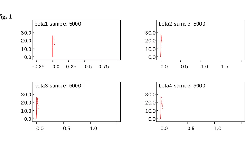
Fig. 1 beta1 sample: 5000

- 0.25 0.0 0.25 0.5 0.75 0.0

10.0 20.0 30.0

beta2 sample: 5000

0.0 0.5 1.0 1.5

0.0 10.0 20.0 30.0

beta3 sample: 5000

0.0 0.5 1.0

0.0 10.0 20.0 30.0

beta4 sample: 5000

0.0 0.5 1.0

(10)

362 beta5 sample: 5000

0.0 0.5 1.0

0.0 10.0 20.0 30.0

Table-1:

node mean sd MC error 2.5% median 97.5% start sample

beta1 0.02767 0.04644 6.596E-4 9.194E-4 0.01824 0.1085 1 5000

beta2 0.0276 0.04951 7.05E-4 8.716E-4 0.01794 0.1101 1 5000

beta3 0.02664 0.03816 4.515E-4 8.512E-4 0.01783 0.1071 1 5000

beta4 0.02709 0.04599 6.905E-4 9.055E-4 0.01795 0.113 1 5000

beta5 0.02739 0.04519 6.082E-4 9.127E-4 0.01816 0.11 1 5000

The graphs and table above are graphs of the posterior distribution of the beta parameters, the graph indicate that the parameters have a distribution which tend to the student t distribution with (n-1) degrees of freedom, n in this case being 5000. However it was observed that the convergence of each of the betas to the t-distribution happen at different rates hence a need to monitor the rate of convergence of each of the parameters to ascertain which of the

parameter will attain the maximum

convergence first, next and last. This will go a long way to determine the variables which should be added or deleted from a model when the number of samples is of interest.

Below are the higher sample sizes which help to

monitor the parameters for general

convergence.

Fig.2

beta1 sample: 10000

0.0 1.0 2.0

0.0 10.0 20.0 30.0

beta2 sample: 10000

0.0 0.5 1.0 1.5

(11)

363 beta3 sample: 10000

0.0 0.5 1.0 1.5

0.0 10.0 20.0 30.0

beta4 sample: 10000

0.0 1.0 2.0

0.0 10.0 20.0 30.0

beta5 sample: 10000

0.0 0.5 1.0 0.0

10.0 20.0 30.0

Table-2: node mean sd MC error 2.5% median 97.5% start sample

beta1 0.02738 0.04891 4.58E-4 9.08E-4 0.01805 0.1132 1 10000

beta2 0.02795 0.05014 4.698E-4 9.614E-4 0.01766 0.1108 1 10000

beta3 0.02762 0.04676 4.937E-4 8.803E-4 0.01796 0.1147 1 10000

beta4 0.02775 0.05019 4.868E-4 8.48E-4 0.01771 0.1145 1 10000

beta5 0.0274 0.04355 3.897E-4 8.313E-4 0.0178 0.1126 1 10000

(12)

364 beta1 sample: 15000

0.0 1.0 2.0

0.0 10.0 20.0 30.0

beta2 sample: 15000

0.0 1.0 2.0

0.0 10.0 20.0 30.0

beta4 sample: 15000

0.0 1.0 2.0

0.0 10.0 20.0 30.0

beta3 sample: 15000

0.0 0.5 1.0 1.5

0.0 10.0 20.0 30.0

beta5 sample: 15000

0.0 1.0 2.0 3.0

0.0 10.0 20.0 30.0

Table-3:

node mean sd MC error 2.5% median 97.5% start sample

beta1 0.02761 0.05053 4.017E-4 8.567E-4 0.01795 0.1126 1 15000

beta2 0.02819 0.05538 4.449E-4 9.546E-4 0.01781 0.113 1 15000

beta3 0.02776 0.04741 3.662E-4 8.578E-4 0.01805 0.1147 1 15000

beta4 0.0278 0.05097 4.135E-4 8.483E-4 0.01785 0.114 1 15000

(13)

365 Fig.4:

beta1 sample: 20000

0.0 1.0 2.0

0.0 10.0 20.0 30.0

beta2 sample: 20000

0.0 1.0 2.0

0.0 10.0 20.0 30.0

beta3 sample: 20000

0.0 0.5 1.0 1.5

0.0 10.0 20.0 30.0

beta4 sample: 20000

0.0 1.0 2.0

0.0 10.0 20.0 30.0

beta5 sample: 20000

0.0 1.0 2.0 3.0

0.0 10.0 20.0 30.0

Table-4:

beta1 0.02761 0.04925 3.264E-4 8.619E-4 0.01803 0.1142 1 20000

beta2 0.02834 0.05407 3.808E-4 9.178E-4 0.018 0.1139 1 20000

beta3 0.02765 0.04569 2.987E-4 8.708E-4 0.01816 0.1136 1 20000

beta4 0.02771 0.04876 3.286E-4 8.79E-4 0.01793 0.1145 1 20000

(14)

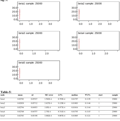
366 fig. 5:

beta1 sample: 25000

0.0 1.0 2.0 3.0

0.0 10.0 20.0 30.0

beta2 sample: 25000

0.0 1.0 2.0 3.0

0.0 10.0 20.0 30.0

beta3 sample: 25000

0.0 1.0 2.0

0.0 10.0 20.0 30.0

beta4 sample: 25000

0.0 1.0 2.0

0.0 10.0 20.0 30.0

beta5 sample: 25000

0.0 1.0 2.0 3.0

0.0 10.0 20.0 30.0

Table-5:

node mean sd MC error 2.5% median 97.5% start sample

beta1 0.02782 0.05527 3.582E-4 8.795E-4 0.01797 0.1139 1 25000

beta2 0.02838 0.05712 3.627E-4 9.129E-4 0.01803 0.1146 1 25000

beta3 0.02794 0.04953 3.05E-4 8.977E-4 0.01816 0.1144 1 25000

beta4 0.02768 0.04757 2.75E-4 8.741E-4 0.01795 0.1143 1 25000

(15)

367 Fig.6:

beta1 sample: 30000

0.0 1.0 2.0 3.0

0.0 10.0 20.0 30.0

beta2 sample: 30000

0.0 1.0 2.0 3.0

0.0 10.0 20.0 30.0

beta3 sample: 30000

0.0 1.0 2.0

0.0 10.0 20.0 30.0

beta4 sample: 30000

0.0 1.0 2.0

0.0 10.0 20.0 30.0

beta5 sample: 30000

0.0 1.0 2.0 3.0

0.0 10.0 20.0 30.0

Table-6:

beta0 0.02827 0.05389 2.925E-4 9.044E-4 0.01815 0.1156 1 30000

beta1 0.02804 0.05706 3.301E-4 8.704E-4 0.01801 0.1142 1 30000

beta2 0.02846 0.05747 3.512E-4 8.849E-4 0.01808 0.1144 1 30000

beta3 0.0282 0.05128 3.101E-4 9.046E-4 0.01823 0.1153 1 30000

beta4 0.02792 0.05196 2.968E-4 8.636E-4 0.01799 0.1143 1 30000

beta5 0.02793 0.05159 2.854E-4 8.762E-4 0.01804 0.1127 1 30000

From the above graphs and tables it will be observed that the convergence to the t- distribution is faster in the parameter beta5, observe the speedy convergence from the 5000 samples to the 15000, this makes it a potential variable for addition in the model. Other parameters converge at greater sample sizes between 10000 and 30000; however the parameters beta3 and beta4 still have room for convergence, for full convergence of these parameters, one might want to consider higher sample sizes. The parameters that converge earliest are potential parameters for addition in the variable selection process.

In the case of the conjugate prior distributions (codes on appendix III and IV), the prior distributions were chosen from a conjugate t distributions having a mean of zero, precision of 0.001 and a degree of freedom of 49, since the initial sample size is 50. The choice of the precision value was chosen to disallow „numerical overflow‟- an error message in WinBUGS which specifies a range of the precision which is inconsistent with the values that may be evaluated by the software.

(16)

368

number of samples increase, the posterior distributions of the beta variates converge to the

Standard t distribution at different rates for each of beta1, beta2, beta3, beta4 and beta5.

Fig.7:

beta1 sample: 5000

-200.0 -100.0 0.0 100.0

0.0 0.005 0.01 0.015

beta2 sample: 5000

-200.0 -100.0 0.0 100.0

0.0 0.005 0.01 0.015

beta3 sample: 5000

-200.0 -100.0 0.0 100.0

0.0 0.005 0.01 0.015

beta4 sample: 5000

-200.0 -100.0 0.0 100.0

0.0 0.005 0.01 0.015

beta5 sample: 5000

-200.0 -100.0 0.0 100.0

0.0 0.005 0.01 0.015

Table-7:

beta1 -0.4019 32.76 0.5362 -64.33 -0.2323 65.5 1 5000

beta2 -0.2515 32.05 0.4629 -61.78 -0.2928 64.04 1 5000

beta3 0.8609 32.12 0.4801 -60.6 0.7065 65.48 1 5000

beta4 -0.2801 32.17 0.5007 -63.1 -0.3354 61.75 1 5000

(17)

369 Fig.8:

beta1 sample: 10000

-200.0 -100.0 0.0 100.0

0.0 0.005 0.01 0.015

beta2 sample: 10000

-200.0 -100.0 0.0 100.0

0.0 0.005 0.01 0.015

beta3 sample: 10000

-200.0 -100.0 0.0 100.0

0.0 0.005 0.01 0.015

beta4 sample: 10000

-200.0 -100.0 0.0 100.0

0.0 0.005 0.01 0.015

beta5 sample: 10000

-200.0 -100.0 0.0 100.0

0.0 0.005 0.01 0.015

Table-8:

beta1 0.01198 32.66 0.383 -63.81 0.2918 65.18 1 10000

beta2 -0.1244 32.21 0.3104 -62.2 -0.5972 63.72 1 10000

beta3 0.216 32.35 0.3393 -61.49 0.2235 64.71 1 10000

beta4 -0.1445 32.37 0.3539 -63.34 -0.1344 62.49 1 10000

beta5 0.2345 32.4 0.3217 -64.39 0.3767 63.3 1 10000

It will be observed at this point that at 5000 samples the beta variates beta1, beta2 and especially beta 5 have distributions that converge to the Standard t distribution faster than that of all the other beta variates. This observation makes them favoured parameters in

our choice of the parameters that will be considered when choosing variables for a reduced model. However the trace of these beta variates are cyclical in nature hence a need to choose just the right amount of samples for pure convergence.

(18)

370 Fig.9:

beta1 sample: 10000

-200.0 -100.0 0.0 100.0

0.0 0.005 0.01 0.015

beta2 sample: 10000

-200.0 -100.0 0.0 100.0

0.0 0.005 0.01 0.015

beta3 sample: 10000

-200.0 -100.0 0.0 100.0

0.0 0.005 0.01 0.015

beta4 sample: 10000

-200.0 -100.0 0.0 100.0

0.0 0.005 0.01 0.015

beta5 sample: 10000

-200.0 -100.0 0.0 100.0

0.0 0.005 0.01 0.015

Table-9:

beta1 0.01198 32.66 0.383 -63.81 0.2918 65.18 1 10000

beta2 -0.1244 32.21 0.3104 -62.2 -0.5972 63.72 1 10000

beta3 0.216 32.35 0.3393 -61.49 0.2235 64.71 1 10000

beta4 -0.1445 32.37 0.3539 -63.34 -0.1344 62.49 1 10000

(19)

371 Fig.10:

beta1 sample: 15000

-200.0 -100.0 0.0 100.0

0.0 0.005 0.01 0.015

beta2 sample: 15000

-200.0 -100.0 0.0 100.0

0.0 0.005 0.01 0.015

beta3 sample: 15000

-200.0 -100.0 0.0 100.0

0.0 0.005 0.01 0.015

beta4 sample: 15000

-200.0 -100.0 0.0 100.0

0.0 0.005 0.01 0.015

beta5 sample: 15000

-200.0 -100.0 0.0 100.0

0.0 0.005 0.01 0.015

Table10:

beta1 -0.03282 32.67 0.2906 -64.44 0.2956 64.67 1 15000

beta2 -0.0372 32.12 0.2567 -63.0 -0.2054 62.96 1 15000

beta3 0.1065 32.29 0.2547 -62.19 -0.1206 64.39 1 15000

beta4 0.07017 32.33 0.2838 -63.11 0.01727 62.93 1 15000

beta5 -0.2541 32.72 0.2668 -64.88 -0.1592 63.65 1 15000

The trace of beta2 are beta 5 are relatively stable at this point while those of beta1, beta3 and beta4 still fluctuate, this is an implication that the convergence of beta2 and beta5 are

(20)

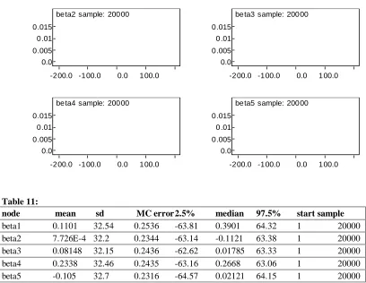
372 Fig.11:

beta2 sample: 20000

-200.0 -100.0 0.0 100.0

0.0 0.005 0.01 0.015

beta3 sample: 20000

-200.0 -100.0 0.0 100.0

0.0 0.005 0.01 0.015

beta4 sample: 20000

-200.0 -100.0 0.0 100.0

0.0 0.005 0.01 0.015

beta5 sample: 20000

-200.0 -100.0 0.0 100.0

0.0 0.005 0.01 0.015

Table 11:

beta1 0.1101 32.54 0.2536 -63.81 0.3901 64.32 1 20000

beta2 7.726E-4 32.2 0.2344 -63.14 -0.1121 63.38 1 20000

beta3 0.08148 32.15 0.2436 -62.62 0.01785 63.33 1 20000

beta4 0.2338 32.46 0.2435 -63.16 0.2668 63.06 1 20000

beta5 -0.105 32.7 0.2316 -64.57 0.02121 64.15 1 20000

At this point, almost all the beta variates have fully converged to the Standard t distribution with beta2 having the least posterior mean (its

(21)

373 Fig.12:

beta1 sample: 25000

-200.0 -100.0 0.0 100.0

0.0 0.005 0.01 0.015

beta2 sample: 25000

-200.0 -100.0 0.0 100.0

0.0 0.005 0.01 0.015

beta3 sample: 25000

-200.0 -100.0 0.0 100.0

0.0 0.005 0.01 0.015

beta4 sample: 25000

-200.0 -100.0 0.0 100.0

0.0 0.005 0.01 0.015

beta5 sample: 25000

-200.0 -100.0 0.0 100.0

0.0 0.005 0.01 0.015

Table-12:

beta1 -0.05494 32.56 0.2107 -64.52 0.1517 64.19 1 25000

beta2 0.03356 32.04 0.2051 -62.56 -0.2061 63.21 1 25000

beta3 0.1144 32.16 0.2314 -62.62 0.1789 63.5 1 25000

beta4 0.2232 32.31 0.2272 -63.1 0.1528 62.93 1 25000

(22)

374 Fig.13:

beta1 sample: 30000

-200.0 -100.0 0.0 100.0

0.0 0.005 0.01 0.015

beta2 sample: 30000

-200.0 -100.0 0.0 100.0

0.0 0.005 0.01 0.015

beta3 sample: 30000

-200.0 -100.0 0.0 100.0

0.0 0.005 0.01 0.015

beta4 sample: 30000

-200.0 -100.0 0.0 100.0

0.0 0.005 0.01 0.015

beta5 sample: 30000

-200.0 -100.0 0.0 100.0

0.0 0.005 0.01 0.015

Table-13:

beta1 -0.09018 32.58 0.1999 -64.64 0.06665 64.45 1 30000

beta2 0.07158 32.12 0.1859 -63.06 -0.091 63.52 1 30000

beta3 0.09854 32.21 0.1995 -62.76 0.1286 63.63 1 30000

beta4 0.04514 32.27 0.2059 -63.26 0.0103 62.73 1 30000

beta5 -0.0461 32.61 0.1816 -64.69 0.08919 63.89 1 30000

The graphs and tables for the 25000 and 30000 sample size iterations show that the speed of convergence increases in the following order beta2, beta3, beta4, beta1 and beta5. In addition, this gives us an insight as to which variables should be added or deleted from a model in the case of variable selection. That is say that the independent variable related to beta2 should be the first to be added to the model and independent variable related to beta5 should be the first to be deleted from the model.

Stochastic Variable Selection

(23)

375

beta0 -0.7453 31.91 0.4071 -64.48 -0.3593 62.36 1 5000

beta1 -0.4697 31.07 0.4074 -61.06 -0.3663 61.41 1 5000

beta2 0.5216 32.14 0.4753 -62.61 0.3092 64.09 1 5000

beta3 0.8325 31.51 0.4714 -59.7 0.8452 61.64 1 5000

beta4 -0.004833 31.79 0.4157 -62.05 -0.1965 60.83 1 5000

beta5 0.1411 32.03 0.3612 -62.58 0.2408 62.41 1 5000

gamma[1] 0.4972 0.5 0.006684 0.0 0.0 1.0 1 5000

gamma[2] 0.5054 0.5 0.007218 0.0 1.0 1.0 1 5000

gamma[3] 0.5052 0.5 0.007145 0.0 1.0 1.0 1 5000

gamma[4] 0.505 0.5 0.006273 0.0 1.0 1.0 1 5000

gamma[5] 0.4942 0.5 0.007286 0.0 0.0 1.0 1 5000

As stated in the section above, the most promising predictors are the ones whose latent

variables have the highest posterior

probabilities, so in the cases above where the stochastic variable selections are used, the latent variables are the γj variables with each

having a Bernoulli distribution (refer to appendix for WinBUGS code). In the case above all the latent variables have similar properties; this is probably due to the fact that all the X‟s (i.e. independent variables) are from a Uniform distribution of the same form.

However the independent variables x2i, x3i, and

x4i associated with β2, β3 and β4 respectively are

choice variables since they have an

approximately equal posterior probability for their latent variables after running an MCMC simulation with 5000 as the sample size. For higher sample sizes, the differences in the latent variables γ may not be easily identified because all the independent variables are from the same Uniform (0, 1) distribution.

Summary

Thus far efforts have been made to establish the relationship between the variables of a linear Bayesian Regression model with special considerations given to the choice of the prior distributions that are being used. The focus of this work is on the possible choices available for the covariates β = (β0, β1, β2, β3, β4, β5) of

the linear Regression model; in addition to choosing the independent variables that are most likely to leave or enter the model in the

case of variable deletion or inclusion

respectively.

In the course of this research work we have been able to briefly explore a brief background of the study with interest on the transition from the classical or frequentist approach to Regression to the more recent Bayesian approach. After studying and proving some of the underlying theories behind the Bayes Regression, we have succeeded at employing two types of prior distribution for the β covariates- the Non-informative (vague) prior distribution and the conjugate prior distribution. In the case of the Non-informative prior distribution, the prior distribution of the beta variates were of the Uniform distribution U(0,σ), this combined with the likelihood function of the Normal distribution (an operation carried out in WinBUGS ) and yielded a t-distribution with mean that is approximately zero and n-1 degrees of freedom for each of the sample sizes n1, . . ., n6 with

n1=5000, n2=10000, n3=15000, n4=20000,

n5=25000 and n6= 30000. In addition the speed

of convergence of each of the each of the beta variates were monitored as an insight to which variables should be added or deleted from the model.

Under the conjugate prior arrangement, the beta variates were drawn from the conjugate t- distribution with mean zero, precision 0.001 and n-1=49 degrees of freedom. This was drawn from an initial sample size of 50. When this was multiplied with the likelihood of the

Normal distribution the result posterior

(24)

376

convergence was also monitored and beta2, beta3, and beta4 were found to potentially variables to be included in the model.

For variable selection, the Stochastic Variable selection was applied using latent variables gamma for each of the beta variates. On the choice of variables, the independent variables associated with beta2, beta3 and bet4 were found to be choice variables for inclusion in the model. This is consistent with the choice of variables selected by simply monitoring the speed of convergence of the beta parameters.

Conclusion

In conclusion it was established that for a Normal linear Regression with the posterior covariates from a t-distribution the appropriate choice of prior distribution would be a vague uniform prior distribution with mean zero and a given standard deviation σ. For a Normal linear Regression model having the posterior beta covariates from Standard t distribution, the most appropriate prior distribution should be from a t-distribution with n-1 degrees of freedom and a zero mean The speed of convergence of the parameters to the desired posterior distribution is an indication of what variables should be added or deleted from models in the case of model reduction. The parameters that converge fastest should have their variables added to the new model.

References

Carlin, B. R. and Chib, S. (1995). “Bayesian Model Choice via Markov Chain Monte Carlo methods” Journal of the Royal Statistical Society B., 57, pp. 473-484.

Chen, M. and Deely, J. J. (1996) “Bayesian Analysis for a Constrained Linear Multiple Regression Problem for Predicting the New Crop of Apples” Journal of Agricultural and Environmental Statistics 1, pp. 467-489.

Congdon P. (2003) Applied Bayesian Modeling, John Wiley &Sons, Ltd,

Dellaportas P. and Stephen A. D. (1995)

“Bayesian analysis of error-in-variables

Regression models” International Biometric Society 51, pp.1085-1095

Dellaportas, P., Forster J. J. and Ntzoufras, I. (1998) “On Bayesian Model and Variable

Selection Using MCMC.”Biometrika 34 pp.11-18

Garthwaite, P. H. and Dickey, J. M. “Elicitation of Prior Distribution for Variable Selection Problems in Regresssion” Annals of Statistics, 20, pp.1697-1719.

George, E. L. And McCulloch, R. E. (1993)

“Variable Selection via Gibbs Sampling” Journal of American Statistical Association 88, pp. 881-889

Goldstein M. (1976) “Bayesian Analysis of Regression Problems” Biometrika trust 63, pp. 51-58

Goldstein M. (1980) “The Linear Bayes Regression Estimation Under Weak Prior Assumptions” biometrika trust 67, pp.621-628.

Hocking, R. R. (1983) “Developments in Linear Regression Methodology” American Statistical Association and America Society for Quality Stable 25, pp 219-230.

Hoeting, J. A., Raftery, A. E., and Madigan, D (2002) Bayesian Variable and Transformation Selection in Linear Regression. “Journal of Computational and Graphical Statistics 11, pp. 485-507

Ishwaran, H and Rao, J. S. (2005) “Spike and Slab Variable Selection: Frequentist and Bayesian Strategies” The Annals of Statistics 33, pp 730-773.

Kuo, L. and Mallick, B. (1998) “Variable Selection for Regression Models.” Sankhya

Lee, M. P. (1983) Bayesian Statistics- An Introduction. Hodder Arnold publishing, New York.

Lindley, D.V. and Smith, A. F. M. (1972)

“Bayes Estimates for the Linear Model” Journal of the Royal Statistical Society Series B 34, pp.1-41

Miller, A. J. (1990) Subset Selection in Regression, London: Chapman & Hall.

Miller, J. A. (2002). Subset Selection in Regression. Boca Raton, Florida, U.S.A.: Chap-man & Hall/CRC.

Mitchell T. J. and Beauchamp J. J. (1988)

“Bayesian Variable Selection in Linear Regression” Journal of the American Statistical Association, 83, pp. 1023-1032.

(25)

377 Nagar A. L. (1960) “A Monte Carlo Study of

Alternative Simultaneous Equations

Estimators.” Econometrica, 28, pp.573-590

O’Hara, R. B. and Sillanpaa M. J. (2009) “A

Review of Bayesian Variable Selection

Methods: What, How and Which” Bayesian Analysis 4, pp. 85-118.

Olubusoye, O. E. and Okewole, D. M. (2009)

“Prior Sensitivity in Bayesian Linear

Regression Model.” Star International Journal (Sciences) 3. pp. 21-29.

Piegorsch W. W. and Casella (1996)

“Empirical Bayes Estimation for Logistic

Regression and Extended Parametric

Regression Models. Journal of Agricultural, Biological and Environmental Statistics 2. pp. 231-249.

Raftery, A. E., Madigan, D. and Hoeting, J. (1997) “Bayesian Model Averaging for Linear Regression Models.” Journal of the American Statistical Association, 92, pp. 179-191

Smith A. F. M. (1973) “A General Bayesian

Linear Model.” Journal of the Royal Statistical Society. Series B (methodological) 35, pp. 67-75.

Smith, M., and Kohn, R. (1996)

“Nonparametric Regression Using Bayesian Variable Selection,” Journal of Econometrics, 75, pp.317-343

Zellner A. (1971) An Introduction to Bayesian Analysis Inference in Econometrics. John Wiley & Sons Ltd.