Dissertation zum Erlangen des akademischen Grades Doktor der Naturwissenschaften der Fakultät für Physik der Ludwig-Maximilians-Universität München
Max-Planck-Institut für Astrophysik
Methods for detecting and characterising
clusters of galaxies
vorgelegt von Björn Malte Schäfer aus Zweibrücken
München, 26.Jan.2005
Dissertation der Fakultät für Physik der Ludwig-Maximilians-Universität München ausgeführt am Max-Planck-Institut für Astrophysik
Vorsitzende: Prof. Dr. Dorothee Schaile 1. Gutachter: Prof. Dr. Matthias Bartelmann 2. Gutachter: Prof. Dr. Simon D.M. White
Beisitzer: Dr. Hans Böhringer
Robert Frost:
On Looking Up By Chance At The Constellations
You’ll wait a long, long time for anything much To happen in heaven beyond the floats of cloud And the Northern Lights that run like tingling nerves. The sun and moon get crossed, but they never touch, Nor strike out fire from each other nor crash out loud. The planets seem to interfere in their curves
Contents
1. Abstract 1
2. Introduction and motivation 3
3. Cosmology and cosmic structure formation 5
3.1. Friedmann-Lemaître cosmological models . . . 5
3.1.1. Cosmological principles and the Robertson-Walker metric . . . 5
3.1.2. Cosmometry . . . 6
3.1.3. Cosmic microwave background . . . 8
3.2. Structure formation . . . 10
3.2.1. Growth of density perturbations in cold dark matter models . . . 10
3.2.2. Numerical simulations of cosmic structure formation . . . 13
3.3. Physics of clusters of galaxies . . . 13
3.3.1. Formation of clusters of galaxies . . . 13
3.3.2. Observational properties of clusters . . . 14
4. PLANCK-surveyor 21 4.1. Introduction to the PLANCK-surveyor . . . 21
4.2. PLANCK mission objectives . . . 21
4.3. Instrument description . . . 22
5. Construction of all-sky thermal and kinetic Sunyaev-Zel’dovich maps 23 5.1. Introduction . . . 23
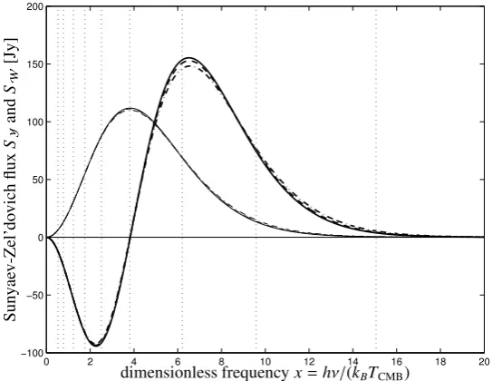
5.2. Sunyaev-Zel’dovich definitions . . . 24
5.3. Simulations . . . 25
5.3.1. Hubble-volume simulation . . . 25
5.3.2. Small scale SPH cluster simulations . . . 26
5.4. Sunyaev-Zel’dovich map construction . . . 26
5.4.1. SZ-template map preparation. . . 26
5.4.2. Cluster selection and scaling relations . . . 28
5.4.3. Projection onto the celestial sphere. . . 29
5.4.4. Completeness of the all-sky SZ-maps . . . 29
5.5. Results. . . 31
5.5.1. Sky views . . . 32
5.5.2. Distribution of angular sizes . . . 35
5.5.3. Distribution of the integrated thermal and kinetic Comptonisation . . . 36
5.5.4. Distribution of Comptonisation per pixel . . . 38
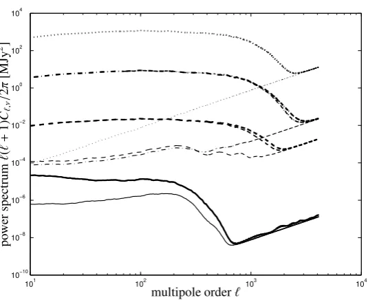
5.5.5. Angular power spectra of the thermal and kinetic SZ-effects . . . 39
5.5.6. Source counts at PLANCK frequencies . . . 40
5.6. Summary . . . 43
6. Microwave emission components of the Milky Way and the Solar system 45 6.1. Introduction . . . 45
6.2. Sunyaev-Zel’dovich definitions . . . 46
6.3.1. Beam shapes . . . 46
6.3.2. Scanning strategy and noise-equivalent maps . . . 48
6.4. Foreground emission components . . . 49
6.4.1. Galactic dust emission . . . 50
6.4.2. Galactic synchrotron emission . . . 51
6.4.3. Galactic free-free emission . . . 51
6.4.4. CO-lines from giant molecular clouds . . . 52
6.4.5. Planetary submillimetric emission . . . 54
6.4.6. Submillimetric emission from asteroids . . . 55
6.4.7. Future work concerning PLANCK’s foregrounds . . . 56
6.5. Simulating SZ-observations by PLANCK . . . 57
6.5.1. SZ-map preparation . . . 58
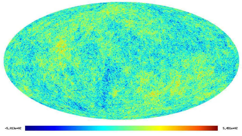
6.5.2. CMB-map generation. . . 58
6.5.3. Preparation of simulation data sets . . . 58
6.5.4. PLANCK-channel correlation properties . . . 61
6.6. Summary and conclusion . . . 62
7. Matched and scale-adaptive multifiltering 65 7.1. Introduction: multi-frequency optimised filtering . . . 65
7.1.1. Assumptions and definitions . . . 66
7.1.2. Concepts in filter construction . . . 67
7.1.3. Matched filter . . . 68
7.1.4. Scale-adaptive filter on the sphere . . . 68
7.1.5. Detection level and gain . . . 69
7.2. Optimised SZ-filters for PLANCK . . . 69
7.2.1. Numerical derivation of filter kernels . . . 69
7.2.2. Discussion of filter kernels . . . 69
7.2.3. Filter renormalisation and synthesis of likelihood maps . . . 76
7.3. Summary and conclusion . . . 79
8. Properties of PLANCK’s SZ-cluster sample 81 8.1. Simulation setup and peak extraction. . . 81
8.1.1. Filter construction and synthesis of likelihood maps. . . 81
8.1.2. Morphology of SZ-clusters in filtered sky-maps . . . 81
8.1.3. Peak extraction and cluster identification . . . 82
8.2. Noise properties and peak statistics. . . 82
8.2.1. Noise in the filtered and co-added maps . . . 82
8.2.2. Detection significances . . . 83
8.3. Cluster detectability as a function of filter parameters . . . 85
8.4. Cluster properties of the recovered SZ-sample . . . 85
8.4.1. Cluster population in the mass-redshift plane . . . 85
8.4.2. Position accuracy of PLANCK’s SZ-clusters . . . 90
8.5. Spatial homogeneity of PLANCK’s SZ-cluster sample . . . 93
8.6. Distribution of peculiar velocities. . . 95
8.7. Summary and conclusion . . . 95
9. A Peano-Hilbert partition for HEALPix tesselated spheres 99 9.1. Motivation. . . 99
9.2. HEALPix tesselation . . . 99
9.3. Peano-Hilbert curves for HEALPix. . . 100
9.4. Properties of the Peano-Hilbert ordering . . . 102
Contents
10.1. Introduction . . . 105
10.2. Sunyaev-Zel’dovich definitions . . . 106
10.3. Wavelets. . . 107
10.3.1. Wavelet definitions . . . 107
10.3.2. Application of wavelets to a cluster profile . . . 107
10.3.3. Analogy to power spectra in Fourier analysis . . . 110
10.4. Simulations . . . 110
10.4.1. SPH cluster simulations . . . 111
10.4.2. SZ-map preparation . . . 111
10.4.3. Cluster selection . . . 111
10.4.4. CMB map generation. . . 113
10.4.5. Simulated single-frequency SZ-observations . . . 114
10.5. Analysis . . . 114
10.5.1. Wavelet basis functions. . . 115
10.5.2. Measurement of wavelet quantities. . . 115
10.5.3. Wavelet spectrum of SZ-cluster maps . . . 116
10.5.4. Correlations with physical quantities. . . 117
10.5.5. Measurement principle . . . 120
10.5.6. Principal component analysis . . . 120
10.5.7. Redshift dependence of the wavelet parameters . . . 121
10.5.8. Noise contributions and their suppression . . . 123
10.5.9. Redshift estimation . . . 126
10.6. Systematics . . . 128
10.6.1. Influence of tilted scaling relations . . . 128
10.6.2. Cool cores of clusters. . . 129
10.6.3. Wavelet analysis of unselected clusters . . . 130
10.7. Redshift estimation in a nutshell . . . 131
10.8. Summary . . . 131
11. Coded mask imaging of extended sources with Gaussian random fields 135 11.1. Introduction . . . 135
11.2. Coded mask imaging . . . 136
11.3. Gaussian random fields . . . 136
11.3.1. Definitions . . . 136
11.3.2. Algorithm. . . 137
11.3.3. Choice of the PSF . . . 137
11.3.4. Scaling applied to the Gaussian random fields . . . 138
11.3.5. Gaussian random fields for circular apertures . . . 138
11.4. Results. . . 139
11.4.1. Visual impression. . . 139
11.4.2. Reproducibility of the PSF . . . 139
11.4.3. Pixel-to-pixel variance . . . 142
11.4.4. Distribution of the pixel amplitudes . . . 142
11.4.5. Partial shadowing. . . 143
11.4.6. Thresholded realisations . . . 143
11.5. Ray-tracing simulations including finite photon statistics . . . 145
11.5.1. Simulation setup . . . 146
11.5.2. Point source sensitivity of a set of Gaussian random fields . . . 147
11.5.3. Sensitivity in observations of extended sources . . . 147
11.5.4. Field-of-view in the observation of point sources . . . 148
11.6. Summary and outlook. . . 149
12.2. Gravitational light deflection . . . 151
12.2.1. Light deflection from Fermat’s principle . . . 151
12.2.2. Cosmological weak lensing . . . 152
12.2.3. Applications of weak lensing in cosmology . . . 153
12.3. Ray-tracing simulations on the large-scale structure . . . 153
12.3.1. A ray-tracing code for cosmological n-body simulations:leica.c. . . 154
12.3.2. Features . . . 155
12.4. Summary and conclusion . . . 155
13. Gravitomagnetic lensing and the integrated Sachs-Wolfe/Rees-Sciama effect 157 13.1. Introduction . . . 157
13.2. Key formulae . . . 158
13.2.1. Structure formation . . . 158
13.2.2. Dark matter currents . . . 159
13.2.3. Limber’s equation for vector fields . . . 159
13.3. Gravitomagnetic lensing . . . 161
13.3.1. Definitions . . . 161
13.3.2. Gravitomagnetic lensing by the large-scale structure . . . 162
13.3.3. Perturbative treatement . . . 163
13.3.4. Corrections to the power spectrum . . . 165
13.3.5. Projected lensing power spectra . . . 165
13.4. Integrated Sachs-Wolfe effect . . . 166
13.4.1. Definitions . . . 167
13.4.2. Connection to the gravitomagnetic potentials . . . 167
13.4.3. Putting the Sachs-Wolfe effect in a cosmological context . . . 168
13.4.4. Perturbative treatment . . . 169
13.4.5. Power spectrum of dark matter currents . . . 169
13.4.6. integrated Sachs-Wolfe angular power spectrum. . . 170
13.5. Summary . . . 171
14. Summary and outlook 173 A. Numerical evaluation of SPH-projections 177 B. Derivation of spherical matched and scale-adaptive filter kernels 181 B.1. Assumptions and definitions . . . 181
B.2. Convolution theorem on the sphere . . . 181
B.3. Concepts of optimised filtering on the sphere . . . 182
B.3.1. Matched filter . . . 183
B.3.2. Scale-adaptive filter. . . 183
C. Integration of Legendre-P`weighted functions 185 D. Integration of Bessel-J` weighted functions 187 D.1. Approximation formulae . . . 187
D.2. Numerical integration . . . 187 E. Decomposition of mixed 3-point correlators of density and velocity fields 189
F. Propagation of photons through gravitomagnetic fields 191
1. Abstract
Methods for detecting and characterising clusters of galaxies
The main theme of this PhD-thesis is the observation of clusters of galaxies at submillimetric wavelengths. The Sunyaev-Zel’dovich (SZ) effect due to interaction of cosmic microwave background (CMB) photons with electrons of the hot intra-cluster medium causes a distinct modulation in the spectrum of the CMB and is a very promising tool for detecting clusters out to very large distances. Especially the European PLANCK-mission, a satellite dedicated to the mapping of CMB anisotropies, will be the first experiment to routinely detect clusters of galaxies by their SZ-signature. This thesis presents an extensive simulation of PLANCK’s SZ-capabilities, that combines all-sky maps of the SZ-effect with a realisation of the fluctuating CMB and submillimetric emission components of the Milky Way and of the Solar system, and takes instrumental issues such as the satellite’s point-spread function, the frequency response, scan paths and detector noise of the receivers into account.
For isolating the weak SZ-signal in the presence of overwhelming spurious components with complicated corre-lation properties across PLANCK’s channels, multifrequency filters based on matched and scale-adaptive filtering have been extended to spherical topologies and applied to simulated data. These filters were shown to efficiently amplify and extract the SZ-signal by combining spatial band-filtering and linear combination of observations at different frequencies, where the filter shapes and the linear combination coefficients follow from the cross- and autocorrelation properties of the sky maps, the anticipated profile of SZ clusters and the known SZ spectral de-pendence. The characterisation of the resulting SZ-sample yielded a total number of 6×10³ detections above a
statistical significance of 3σand the distribution of detected clusters in mass, redshift, and position on the sky. In a related project, a method of constructing morphological distance estimators for resolved SZ cluster images is proposed. This method measures a cluster’s SZ-morphology by wavelet decomposition. It was shown that the spectrum of wavelet moments can be modeled by elementary functions and has characteristic properties that are non-degenerate and indicative of cluster distance. Distance accuracies following from a maximum likelihood approach yielded values as good as 5% for the relative deviation, and deteriorate only slightly when noise components such as instrumental noise or CMB fluctuations were added. Other complications like cool cores of clusters and finite instrumental resolution were shown not to affect the wavelet distance estimation method significantly.
Another line of research is the Rees-Sciama (RS) effect, which is due to gravitational interaction of CMB photons with non-stationary potential wells. This effect was shown to be a second order gravitational lensing effect arising in the post-Newtonian expansion of general relativity and measures the divergence of gravitomagnetic potentials integrated along the line-of-sight. The spatial autocorrelation function of the Rees-Sciama effect was derived in per-turbation theory and projected to yield the angular autocorrelation function while taking care of the differing time evolution of the various terms emerging in the perturbation expansion. The RS-effect was shown to be detectable by PLANCK as a correction to the primordial CMB power spectrum at low multipoles. Within the same perturbative formalism, the gravitomagnetic corrections to the autocorrelation function of weak gravitational lensing observ-ables such as cosmic shear could be determined. It was shown that those corrections are most important on the largest scales beyond 1 Gpc, which are difficult to access observationally. For contemporary weak lensing surveys, gravitomagnetic corrections were confirmed not play a significant role.
Methoden zum Aufspüren und Charakterisieren von Galaxienhaufen
Das zentrale Thema dieser Dissertation ist die Beobachtung von Galaxienhaufen bei Millimeter-Wellenlängen. Der Sunyaev-Zel’dovich (SZ) Effekt, der durch die Wechselwirkung der Photonen des kosmischen Mikrowellenhinter-grundes (CMB) mit Elektronen des heißen intra-Cluster Mediums im Zentrum von Galaxienhaufen hervorgerufen wird, verursacht eine Modulation des CMB-Spektrums und ist eine sehr vielversprechende Technik, Galaxien-haufen bis zu sehr großen Abständen zu entdecken. Vor allem der europäische PLANCK-Satellit, der die Kartogra-phie der CMB-Anisotropien zur Aufgabe hat, wird das erste Observatorium sein, das routinemäßig Galaxienhaufen durch ihre SZ-Signatur aufspürt. In dieser Dissertation wird eine detaillierte Simulation der SZ-Beobachtungen mit PLANCK beschrieben, die Himmelskarten des SZ-Effekts mit Fluktuationen des Mikrowellenhintergrundes und Vordergrundemissionen der Milchstraße und des Sonnensystems verbindet. Instrumentelle Komplikationen wie die Ortsauflösung der Optik, die Frequenzfenster der Radioempfänger, das Scan-Muster und das Detektorrauschen wurden berücksichtigt.
Um das schwache SZ-Signal zu isolieren, das durch die um ein Vielfaches stärkeren Vordergründe überdeckt ist, wurden Multifrequenz-Filter basierend auf dem matched filter- und dem scale-adaptive filter-Algorithmus auf sphärische Topologien erweitert und auf die simulierten Daten angewendet. Es wurde gezeigt, dass diese Filter das SZ-Signal effizient verstärken und extrahieren können, was durch die Kombination von räumlichen Filtern und Lin-earkombination verschiedener Karten geschieht. Die Filterformen und Koeffizienten der Linearkombination folgen aus den Kreuz- und Autokorrelationseigenschaften der Himmelskarten, dem erwarteten SZ-Profil der Galaxien-haufen und dem bekannten spektralen Verlauf des SZ-Effekts. Der resultierende SZ-Katalog, der 4×10³Einträge mit Signifikanzen größer als 3σumfasst, wurde in Bezug auf die Verteilung der detektierten Galaxienhaufen in Masse, Rotverschiebung und Position untersucht.
In einem verwandten Projekt stelle ich eine Methode vor, mittels derer der Abstand eines SZ-Galaxienhaufens durch seine Morphologie abgeschätzt werden kann. In dieser Methode wird die Morphologie eines Galaxienhaufens durch Wavelets analysiert. Es konnte gezeigt werden, dass das Spektrum der Wavelet-Momente durch elementare Funktionen beschrieben werden kann und charakteristische Eigenschaften hat, die nicht-entartet sind und Indika-toren für den Abstand des Galaxienhaufens sind. Die Genauigkeit der Abstandsmessung, die wahrscheinlichkeits-theoretisch bestimmt wurde, ergibt Werte von 5% für die relative Abweichung, wobei sich diese Zahl nur marginal verschlechtert, wenn Rauschkomponenten wie instrumentelles Rauschen oder CMB-Fluktuationen berücksichtigt werden. Es konnte gezeigt werden, dass andere Komplikationen, wie abgekühlte Kerne von Galaxienhaufen oder die endliche Ortsauflösung der Detektoren, diese Methode nicht stark beeinflussen.
Ein anderes Forschungsgebiet ist der Rees-Sciama (RS) Effekt, der durch gravitative Wechselwirkung der CMB-Photonen mit zeitlich veränderlichen Gravitationsfeldern verursacht wird. Dieser Effekt konnte auf einen Gravita-tionslinseneffekt zweiter Ordnung zurückgeführt werden, der in der post-Newtonschen Entwicklung der Formeln der allgemeinen Relativitätstheorie erscheint. In dieser Darstellung misst der RS-Effekt die Divergenz der gravit-omagnetischen Potenziale entlang der Sichtlinie. In dieser Beschreibung wurde die Autokorrelationsfunktion des RS-Effekts in Störungsrechnung hergeleitet und projiziert, um die Winkel-Autokorrelationsfunktion zu erhalten, während die verschiedenen Zeitentwicklungen der Terme in der Störungsreihe berücksichtigt wurden. Der RS-Effekt sollte von PLANCK als Korrektur zur Autokorrelationsfunktion des primordialen CMB auf grossen Winkel-skalen detektierbar sein. Innerhalb des gleichen Formalismus habe ich gravitomagnetische Korrekturen zu der Autokorrelationsfunktion beliebiger Gravitationslinsengrößen bestimmt, die auf den größten Skalen jenseits von 1 Gpc wichtig werden sollten, allerdings Experimenten nur schwer zugänglich sind. Auf Skalen, die durch laufende Durchmusterungen untersucht werden, spielen gravitomagnetische Korrekturen nur eine untergeordnete Rolle.
2. Introduction and motivation
The last couple of decades has witnessed the evolution of cosmology from a philosophical to a sound scientific discipline. The first observational fact was E. Hubble’s discovery of the recession velocity of galaxies, which he found to be proportional to their distance. This suggested that space itself is expanding and not static. World models in the framework of general relativity based on solutions of Friedmann’s equations were found by A. Einstein and W. de Sitter which explain the universal expansion. R. Alpher, H. Bethe and G. Gamov investigated the thermal history of an expanding Universe and realised that the early Universe was hot and dense enough to allow thermonu-clear synthesis of light elements. Their theory was supported by measurements of the cosmic abundance of light elements, in particular of deuterium. A further prediction of their work was the cosmic background radiation, which was succesively detected by A. A. Penzias and R. W. Wilson.
Today, the parameters describing the homogeneous dynamics of the Universe are known on the percent level and cosmology turned to answering the question of structure formation. Fluctuations in the sky temperature of the cosmic microwave background suggested that the structures such as galaxies and clusters of galaxies form by gravitational amplification from these tiny primordial seed fluctuations which was suggested by I. Novikov and Y. B. Zel’dovich. J. Peebles proposed that most of the matter was not electromagnetically interacting (dark matter) and that the structure formed by gravitational aggregation of this newly introduced fluid, which mended a number of problems baryonic models of structure growth were unable to overcome. It was then proposed by J. P. Ostriker, M. Rees and S. D. M. White that luminous objects like galaxies form inside dark matter structures by condensation and cooling of baryons. In this thesis, Chapter 3provides a summary of the key results of cosmology, structure formation and cluster physics.
Theories of cosmic structure formation can be tested in a number of ways. In modern cosmology the statistical properties of the dark matter field or any tracer of it like the spatial distribution of baryons or galaxies as tracer particles are described in terms of its n-point correlation function. The correlation functions are observationally accessible by various experiments. Classically, the large-scale distribution of galaxies was the first to be investigated and continues to be a very interesting technique. In particular, it yields information about the clustering of dark matter on small scales and the transition from linear to nonlinear structure formation, where perturbation theory ceases to be applicable. Another observational channel is the X-ray band: Clusters of galaxies are powerful emitters of X-ray radiation and X-ray surveys are able to determine the fluctuations of the density field by investiating its peak statistics on the cluster separation scale. Furthermore, X-rays probe the distribution of baryons inside dark matter halos and investigate processes like radiative cooling, feedback and metal enrichment which strongly influences the baryonic morphology of a cluster.
All these observations are aiming at the determination of cosmological parameters related to structure formation to a level of accuracy comparable to the parameters governing the homogeneous dynamics of the Universe. Ob-servations of the dynamics of the large-scale structure are complemented by numerical computer simulations of structure growth. In these models, the equations of structure formation (the equation of continuity, Euler’s equation and Laplace’s equation) are solved for a discretised density field. Despite the fact that these simulations are very challenging from the algorithmic and computational point of view, they yield valuable insight into dark matter dy-namics in the nonlinear stages of structure evolution, halo formation and baryonic physics in the centres of galaxies and clusters of galaxies. The core theme of this thesis is the derivation of observational properties of the large-scale structure from numerical simulations. Of special interest to this thesis is the simulation of clusters of galaxies in a new observational window: The thermal Sunyaev-Zel’dovich effect predicts that clusters of galaxies leave a trace in the spectrum of the cosmic microwave background radiation by Compton interaction of the electrons of the hot-intra cluster medium with photons of the microwave background. Recent advances in submillimetric receiver technology made the detection of this small effect possible.
objectives is given in Chapter4. PLANCK will be the first observatory to routinely detect clusters of galaxies by their SZ-signature. The SZ-effect is a particularly promising tool for investigating clusters of galaxies because clusters can be detected out to very large distances, possibly out to redshifts of unity as analytic estimates suggest. Chapters5through8describe a very detailed simulation of PLANCK’s SZ-capabilities which includes many aspects of cluster formation and distribution, baryonic physics and asymmetric SZ-morphologies, Galactic and ecliptic foregrounds and many instrumental imperfections such as receiver noise, frequency response and resolution of the optical system. The weak SZ-signal is amplified and extracted by matched and scale-adaptive filtering, which has been extended to spherical topologies and multi-frequency observations.
In Chapter10, I propose a method of constructing morphological distance estimators for resolved SZ cluster im-ages. This method measures a cluster’s SZ-morphology by wavelet decomposition. It is shown that the spectrum of wavelet moments can be modeled by elementary functions and has characteristic properties that are non-degenerate and indicative of cluster distance. Distance accuracies following from a maximum likelihood approach yielded values as good as 5% for the relative deviation, and deteriorate only slightly when noise components such as instru-mental noise or CMB fluctuations were added. Other complications like cool cores of clusters and finite instruinstru-mental resolution were shown not to affect the wavelet distance estimation method significantly. This method will be of particular use in future dedicated high-yield SZ-surveys in order to select targets for optical or X-ray follow-up observations.
Chapter9 is more technical in nature. A central quantity in CMB data analysis tasks is the pairwise pixel co-variance matrix, which contains information about non-isotropic and non-Gaussian noise components and is a key quantity in map reconstruction, component separation and foreground subtraction. For usual pixel numberings in the HEALPix tesselation of the sphere, which is commonly used in CMB data analysis, the covariance matrix has a very complicated shape. I propose to number the pixels along a fractal, self-similar Peano-Hilbert curve that can be constructed for all HEALPix resolutions. Using this numbering, the covariance matrix assumes a band-diagonal shape which makes the computation of the determinant and matrix inversion possible.
A byproduct of the simulation of CMB fluctuations on the basis of Gaussian random fields was a new way of generating coded mask pattern for X-ray andγ-ray imaging, which is described in Chapter11. Coded mask cam-eras observe a source by recording the shadow cast by a mask onto a position-sensitive detector. The distribution of sources can be reconstructed from this shadowgram by correlation techniques. By using Gaussian random fields, coded mask patterns can be specifically tailored for a predefined point-spread function which yields significant ad-vantages with respect to sensitivity in the observation of extended sources while providing a moderate performance compared to traditional mask generation schemes in the observation of point sources. Coded mask patterns encod-ing Gaussian point-spread functions have been subjected to extensive ray-tracencod-ing studies where their performance has been evaluated.
Another experimental tool for investigating the correlation properties of the cosmic density field is gravitational lensing. Gravitational interaction of photons with the large-scale structure induces tiny distortions in the images of background galaxies which can nowadays be measured reliably. There exist mathematical tools that link the angular correlation properties of the distorted galaxy images to the spatial correlation properties of the dark matter density field, in particular the amplitude of the correlation function. In Chapter12I describe a ray-tracing code for comput-ing lensed photon geodesics on density fields followcomput-ing from cosmological simulations of structure formation. This code covers many aspects of gravitational lensing and is able to derive lensing data from cosmological simulation at a high level of authenticity.
3. Cosmology and cosmic structure formation
Abstract
This chapter provides an introduction to the theory of cosmic structure formation, and the key concepts of modern cosmology as relevant for this work. After summarising Friedmann-Lemaître cosmological models in Sect.3.1, the theory of cosmological structure formation and the description of the statistical properties of the large-scale structure by means of correlation functions is presented in Sect.3.2. Various aspects of the physics of clusters of galaxies, e.g. their formation and their properties in different observational channels are discussed in Sect.3.3.
3.1. Friedmann-Lemaître cosmological models
3.1.1. Cosmological principles and the Robertson-Walker metric
3.1.1.1. Relativistic world models
In general relativistic world models, events are described by their world coordinates, a 4-tuple containing the time coordinate and three spatial coordinates. The infinitesimal distance ds between two events differing in coordinates by dxµcan be computed with the metric tensor gµν, ds2 = g
µνdxµdxν. In general relativity, the metricgµν is a dynamical field, which is determined by Einstein’s field equation (Landau & Lifshitz 1975),
Rµν−R
2gµν≡Gµν = 8πG
c4 Tµν+ Λgµν, with Tµν =
ρ+ p c2
υµυν−pgµν, (3.1)
where the energy momentum tensor composed of the densityρand pressure p of the cosmological fluids moving with 4-velocitiesυµacts as a source term. The Einstein-tensor Gµνis formed from the Ricci tensor Rµνand the Ricci scalar R, which are contractions of the Riemann tensor Rκλµν, i.e. of the second derivatives of the metricgµν. Hence, formula3.1is a generalised Poisson equation. In eqn.3.1,Λdenotes the cosmological constant.
3.1.1.2. Cosmological principle
In order to make an ansatz for the metric tensorgµνand to find a spherically symmetric solution of Einstein’s field
equation 3.1that describes the expansion dynamics of the Universe, the cosmological principle was introduced. This principle requires isotropy and homogeneity:
• When averaged over sufficiently large scales, there exists a mean motion of matter and radiation in the Uni-verse. From a frame of reference comoving with this mean motion, all averaged observables appear to be isotropic.
• All (imaginary) observers who follow this mean motion experience the same history of the Universe and measure the same values for all averaged observables.
3.1.1.3. Robertson-Walker line element
The spatial coordinates of an observer at rest in the comoving frame, from which the mean motion of radiation and matter appears isotropic, are constant, dxi=0 and hence ds2=g
00dt2. It follows from the postulate of isotropy that
clocks can be synchronised in a way that space-time components of the metric tensorg0ivanish. The line element
satisfying the cosmological postulates can be written:
wheregi jare the spatial components of the metric tensor. In order to conserve homogeneity the spatial part of the metric is only allowed to scale with a function a(t) depending on cosmic time t, giving:
ds2 =c2dt2−a2(t)dr2, (3.3)
where dr is the line element on spatial hypersurfaces. Introducing spherical coordinates r = (w, θ, φ) gives the Robertson-Walker line element for homogeneous and isotropic spaces:
ds2=c2dt2−a2(t)hdw2+fK2(w)dθ2+sin2θdφ2i. (3.4) Homogeneity requires, that the function fK(w) is either trigonometric for positive values of the curvature K, linear for vanishing K or hyperbolic for negative K:
fK(w)=
1 √ Ksin √
Kw ,K>0, spherical,
w ,K=0, flat,
1
√ |K|sinh
√
|K|w,K<0, hyperbolic.
(3.5)
3.1.1.4. Redshift
Due to the expansion of the Universe, photons are redshifted during their propagation from their source to the observer. In general, the redshift z of an object is the fractional Doppler shift of its light resulting from radial motion with velocityυ:
z≡λo
λs −1−→1+z=
s
1+υ/c
1−υ/c, (3.6)
whereλsis the wavelength of the emitted andλoof the observed radiation. In cosmology, the Doppler shift is due to emitter’s recession with the Hubble flow and thus related to the ratio of scale factors a at the times of emission and absorption: 1+z= ao
as. For an observer at zo=0 and source zs=z, the formula becomes a=1/(1+z)↔z=1/a−1.
3.1.2. Cosmometry
3.1.2.1. Friedmann’s equations and the adiabatic equation
Solving Einstein’s field equation3.1with the Robertson-Walker metric3.4as an ansatz forgµνfor a homogeneous
perfect fluid leads to Friedmann’s equations (Friedmann 1922,1924): ˙a
a = r
8πG 3 ρ−K
c2
a2 +
Λ 3 and
¨a a =−
4πG 3 ρ+
3p c2
!
+Λ
3, (3.7)
which describe the time evolution of the scale factor a(t) depending on the properties of the cosmological fluids. The two Friedmann equations can be combined to form the adiabatic equation,
d dt
h
a3(t) c2ρ(t)i+p(t)d dta
3(t)=0, (3.8)
which describes the time evolution of the energy content of a volume that is expanding with the Hubble flow. The change in internal energy da3c2ρin a volume is equal to the pdV-work, i.e. the pressure times the change in proper volume. For that reason, the adiabatic equation corresponds to the first law of thermodynamics applied to the cosmological expansion.The Hubble function H(t) is defined as the logarithmic derivative of a(t):
H(t)≡ d
dtln(a)= ˙a a −→H
2(t)=H2 0
" ΩR
a4(t) +
ΩM a3(t)+
ΩK a2(t) + ΩΛ
#
. (3.9)
The value of H0is one of the least accurately known cosmological parameters, but measurements of CMB anisotropies
(Spergel et al. 2003) and from Cepheid variable stars in distant galaxies (the Hubble key project, Freedman et al. 2001) seem to converge to a value of H0=100 h kms−1Mpc−1with h'0.7. The combination
3H02
3.1.2 Cosmometry
is the critical density of the Universe. If in a cosmological model all densities add up toρcrit, spatial hypersurfaces
are flat and the curvature K vanishes. The energy density of all cosmological fluids (radiation 3p/c2, matterρ,
curvature K and the cosmological constantΛ) can be expressed in units ofρcritto yield:
ΩR= 8πG p c2H2
0
, ΩM=ρρ
crit
, ΩK= Kc2 H2
0
, ΩΛ= Λ
3H2 0
, etc. (3.11)
For filling in the suspiciously looking gap in the Hubble function H for the a−1(t) term, a new fieldφ
Qrefered to as quintessence with the densityΩQhas been invented (Wetterich 1988,Ratra & Peebles 1988,Wetterich 1995,Doran & Wetterich 2003) and generalised by using a specific choice of the self-interaction potential V(φQ) to mimick
arbitrary dependences on the scale factor a. Today’s most accurate measurements of the density parameters have been carried out by the WMAP satellite (Spergel et al. 2003). Reference values are matter densityΩM=0.27±0.04, baryonic densityΩB =0.044±0.004, curvatureΩK =0.02±0.02 and cosmological constantΩΛ=0.73±0.04. The radiation densityΩRdoes not play a role in cosmic dynamics after decoupling due to its fast decrease with a. 3.1.2.2. Distances in cosmology
In curved and non-stationary space-time, distances are no longer unique and different distance measurement pre-scriptions lead to different distance measures. In general relativity, distance measures relate the positions of two events on two separate geodesic lines, which intersect a common light cone centered on an observer (Bartelmann & Schneider 2001,Hogg 1999). The proper time dP(zs,zo) is defined to be the light travel time of a signal emitted by a source at redshift zsto an observer at zo<zs: ddP=−cdt. Inserting the Hubble function yields ddP=−cda/(aH)
and finally:
dP(zo,zs)= c H0
Z a(zo)
a(zs)
da ha−1ΩM+ ΩK+a2ΩΛi−
1 2.
(3.12) The comoving distance, which is a very important distance measure in gravitational lensing and simulations of structure formation, is defined to be the distance on the spatial hyper-surface at time t between the world lines of source and observer comoving with the Hubble flow. Light travels along the geodesic, ds=0, hence cdt=−addC.
Replacing dt as before by inserting the Hubble function H gives ddC=−cdt/a=−cda/(a2H):
dC(zo,zs)= c H0
Z a(zo)
a(zs)
da haΩM+a2ΩK+a4ΩΛi−
1
2. (3.13)
The comoving distance with the observer at z=0 is refered to asw(z)≡dC(zo,zs). Yet another distance measure is the angular diameter distance dA(zs,zo), which relates the physical size∆L of an object at redshift zsto its angular size∆αas seen from an observer at redshift zo,∆αdA = ∆L. The angular size of a yardstick placed at zs should decrease proportional to a(zs) fK(w(zs)), where fK(w(zs)) is the radial coordinate distance between observer and object, and a(zs) is the scale factor at the time of light emission, which gives:
dA(zo,zs)=a(zs) fK[dC(zo,zs)]. (3.14)
Due to the factor a(zs), the angular diameter distance is not additive. The luminosity distance dL(zs,zo) relates the luminosity of a source at zsto the flux received by an observer at zo.
dL(zo,zs)=
a(zo) a(zs)
!2
dA(zs,zo)=
a(zo)2
a(zs)
fK[dC(zo,zs)]. (3.15)
The luminosity distance is proportional to the angular diameter distance, which relates the physical area of a source at zsto its apparent solid angle, as seen from the observer at zo. The energy flux is further diminished, because the photons are redshifted by ao/zsand the difference in arrival times of two photons is stretched by ao/zs, giving the final formula. The various distance measures as a function of redshift z are compared in Fig.3.1.
From these distance measures, only dP, dCand dLare monotonic in a and z. Furthermore, only dC(z) and dP(z)
are additive, which follows from the relationRzz3
1 da di(a)=
Rz2
z1 da di(a)+
Rz3
z2 da di(a). Yet another distance measure
10−2 10−1 100 101 102 103 100
101 102 103 104 105
106
107
PSfrag replacements
redshiftz
distance
di
[Mpc
/
h
]
Figure 3.1.: Distance measures in cosmology: The comoving distance dC(z)=w(z) (solid line), the proper distance dP(z)
(dashed line), the angular diameter distance dA(z) (dash-dotted line) and the luminosity distance dL(z) (dotted line).
3.1.3. Cosmic microwave background
3.1.3.1. Cosmic microwave background radiation
The cosmic microwave background (CMB) originated in the early hot phase of the Universe, when photons were created in thermal equilibrium with electromagnetically interacting particles (Dicke et al. 1965). With the Hubble expansion, the Universe cooled adiabatically. The adiabatic index of relativistic particles isγ = 4/3 (Shapiro & Teukolsky 1983), which yields for the adiabatic expansion T ∝V1−γ ∝a. During the expansion, photons remained in thermal equilibrium until the temperature was sufficiently low for the electrons to combine with protons and α-particles to form hydrogen and helium. The photons decoupled from the matter constituents due to the rapidly decreasing abundance of charged particles. In this way, the Universe became transparent for radiation at a redshift of z'103. The photons retained their Planckian spectrum they had acquired while they were in thermal equilibrium
with the electron-positron plasma, and the temperature decreased in proportion with the scale factor. The relic radiation was detected byPenzias & Wilson(1965) and is nowadays proved to have a black body spectrum with TCMB =2.725 K (Fixsen et al. 1996) to very high accuracy.
The CMB shows tiny temperature anisotropies (∆T/T '10−5) imprinted by density perturbations present at the time of decoupling through various mechanisms (Hu 1995,Giovannini 2004). The physics governing the behaviour of a volume element of electron-proton plasma coupled to a radiation field is an interplay between gravity and radiation pressure. Photons released in overdense regions are redshifted because they have to climb out potential wells and hence they are cooler than the average CMB temperature. This effect, first examined bySachs & Wolfe
(1967), probes the potential fluctuations (and hence the density fluctuations) on the surface of last scattering. On scales smaller than the sound horizon, radiation pressure is able to provide a restoring force against the pull of gravity. The plasma-photon fluid is thus carrying out oscillations, which are excited when the size of the perturbation is equal to the horizon. At fixed physical scale, these oscillations are coherent, giving rise to distinct peaks in the CMB power spectrum. On the smallest scales, density perturbations can be destroyed if the radiation pressure exceeds the self-gravity.
3.1.3 Cosmic microwave background
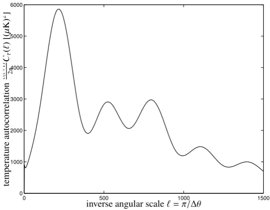
0 500 1000 1500
0 1000 2000 3000 4000 5000 6000
PSfrag replacements
inverse angular scale`=π/∆θ
temperature
autocorrelation
`
(
`
+
1)
2
π
Cτ
(
`
)[(
µ
K)
2 ]
Figure 3.2.: The angular power spectrum Cτ(`) of the fluctuations in the cosmic microwave backgroundτ(θ), for the
ΛCDM model, withΩM =0.3,ΩB=0.04 andΩΛ=0.7.
primary subject of this thesis.
3.1.3.2. Statistical description of the CMB: Gaussian random fields
Due to their Gaussianity, the CMB temperature fluctuations τ(θ) can be decomposed into spherical harmonics Y`m(θ, ϕ), which form a harmonic system of functions, because they are solutions to Laplace’s equation in spherical
coordinates:
τ`m=
Z
4π
dΩτ(θ)Y`∗m(θ)↔τ(θ)= ∞ X
`=0 +`
X
m=−`
τ`mY`m(θ) with Y`m=
r
2`+1 4π
s
(`− |m|)!
(`+|m|)!P`m(cosθ)e
imϕ. (3.16)
From theτ`m-coefficients, the angular power spectrum Cτ(`) can be obtained by averaging over all 2`+1 values of m at given multipole order`, i.e. at fixed anguar scale∆θ'π/`:
Cτ(`)≡2`1
+1
+`
X
m=−`
τ`mτ∗`m. (3.17)
Provided that the CMB fluctuations are indeed a Gaussian random field, all statistical information is contained in Cτ(`). Current CMB data is subjected to a plethora of techniques aiming at the amplification and detection of
non-Gaussian features. Most of the analyses find the CMB to be consistent with non-Gaussianity (Komatsu et al. 2003), but interesting non-Gaussian features should be present, the most notable being gravitational lensing of the CMB (Hu 2000b,Hamana et al. 2004).
The angular power spectrum Cτ(`) as a function of inverse angular scale`'π/∆θof the CMB fluctuationsτ(θ) is depicted in Fig.3.2for aΛCDM model. By using cosmological Boltzmann codes (Seljak & Zaldarriaga 1996,
Lewis et al. 2000,Hu 2000a), the power spectrum Cτ(`) can be computed for a given set of cosmological parameters.
By inversion, measurements of Cτ(`) are powerful probes of the cosmology, especially the geometry of the universe
in terms of the curvatureΩK. Furthermore, Cτ(`) provides important information about the statistics of fluctuations
3.1.3.3. Cosmic neutrino background
In analogy to the CMB, there is a background of relic neutrinos from the era of nucleosynthesis in the early universe at redshifts of z'1010, that decoupled at temperatures of kBT '1 MeV, because at this stage, the time scale of
leptonic interactions became larger than the expansion time scale of the Universe. The neutrinos from this cosmic neutrino background are expected to have Fermi-Dirac spectrum with an equilibrium temperature of TCNB=1.95K.
3.2. Structure formation
3.2.1. Growth of density perturbations in cold dark matter models
3.2.1.1. Properties of dark matter
The current models of structure formation require the majority of matter not to couple to photons and to interact only by gravity. The most stringent observation which requires the matter to be dark, i.e. not interacting electro-magnetically is the formation of structure since the emergence of the CMB, apart from rotation curves of spiral galaxies, gravitational microlensing or discrepancies of mass estimates of clusters of galaxies by application of the virial theorem compared to sum of masses of the cluster’s member galaxies and the intra-cluster medium.
Dark matter is believed to be a yet undiscovered gravitationally interacting elementary particle, that neither carries electromagnetic, nor strong charges, but possibly interacts by the weak nuclear force. There is a large industry of experiments aiming at a direct detection of dark matter particles (CDMS1, DAMA2, GENIUS3, EDELWEISS4), but
it is doubtful whether their sensitivity is sufficiently high. Dark matter interacts solely by gravity and is thought to have a vanishing cross section for collisions with other dark matter particles, which impacts on the central structure of gravitationally bound objects. Self-interacting dark matter influences the core structure of dark matter haloes (Yoshida et al. 2000) or could be detected by its annihilation signal (Stöhr et al. 2003). At the time of their de-coupling from weak interactions, the dark matter particles were non-relativistic, i.e. cold, which has important implications on structure formation. The standard model of cosmological structure formation assumes the existence of initial seed fluctuations in the dark-matter distribution, which grew by gravitational attraction. A possible mech-anism for producing these seed fluctuation are quantum fluctuations in the early universe, which were stretched to cosmological size by inflation.
3.2.1.2. Linear growth
Perturbations in the dark matter density fieldρ(x,t) are described by the density contrastδ(x,a): δ(x,a)= ρ(x,a)− hρ(a)i
hρ(a)i , (3.18)
with the average cosmic densityhρ(a)i= ΩMρcrita−3. By using (relativistic) perturbation theory, it can be shown that
in the linear regime|δ| 1 perturbations grow differently with a, depending which fluid dominates the cosmological dynamics, as long as the Einstein-de Sitter limit is fulfilled, i.e.ΩM(a)'1:
δ(a)∝
(
a2 ,a<a
eq, radiation dominated era,
a ,a>aeq, matter dominated era.
(3.19)
At late times, when either the matter densityΩM has decreased sufficiently or the cosmological ΩΛhas started dominating the Hubble expansion, the linear growth depends on time a according to:
δ(a) δ(1) =a
g0(a)
g0(1) ≡D+(a). (3.20)
1http://cdms.berkeley.edu/
2http://www.lngs.infn.it/lngs/htexts/dama/welcome.html
3.2.1 Growth of density perturbations in cold dark matter models
0 0.1 0.2 0.3 0.4 0.5 0.6 0.7 0.8 0.9 1
0 0.1 0.2 0.3 0.4 0.5 0.6 0.7 0.8 0.9 1
PSfrag replacements
scale factora
gro
wth
function
D+
(
a
)
Figure 3.3.: The growth function D+(a) for theΛCDM model (solid line), the SCDM model (dash-dotted line) and a
low-density model withΩM=0.3 and vanishing cosmological constantΩΛ=0.0 (dashed line).
A phenomenological fit tog0(a) for theΩM-dominated phase of structure growth is provided byCarroll et al.(1992): g0(a)=5
2ΩM(a)
"
Ω4/7
M (a)−ΩΛ(a)+ 1+ 1 2ΩM(a)
!
1+ 1 70ΩΛ(a)
!#−1
. (3.21)
The growth function D+(a) as a function of scale factor a of theΛCDM model, the SCDM model and a low density model without cosmological constantΛis depicted in Fig.3.3.
3.2.1.3. 2-point statistics, initial conditions and the shape ofPδ(k)
The density fluctuations δ(x) are assumed to be Gaussian, and can be completely characterised by their power spectrum Pδ(k), which is defined by:
hδ(k)δ∗(k0)i=(2π)3δD(k−k0)P
δ(k), (3.22)
with the Fourier transform δ(k) = R d3xδ(x) exp(−ikx). In linear perturbation theory, the density field grows
homogeneously, hence individual Fourier components evolve independently:
δ(x,a)=D+(a)δ(x)−→δ(k,a)=D+(a)δ(k), (3.23) as long as the wavelength of the perturbation is small compared to the comoving horizon size. dH=c/[aH(a)], i.e.
the distance which a photon can cover since the big bang.
It is commonly assumed that the power spectrum Pδ(k) is scale invariant on large scales, Pδ(k)∝knswith ns'1 (Harrison 1970,Peebles & Yu 1970,Zeldovich 1972). On small scales, the growth of structure is suppressed by the fast radiation driven expansion at early times. A perturbation in δ, which has the wavelengthλ = 2π/k can start growing at the cosmic epoch astart ifλis smaller than the horizon size at that epoch,λ < dH(astart). But at early
times, the expansion time scale tHubbleis smaller than the collapse time scale tDM:
tHubble∝
1 √
GρR < 1 √
GρM ∝tDM, (3.24)
due toρR > ρMand the growth of the perturbation stalls. This suppression is effective from astartuntil the epoch of
fluctuations withλ < dH(aeq) are suppressed by (astart/aeq)2. Now, the time astartis a function of the wavelength
of the fluctuation, byλ = dH(astart). In the Einstein-de Sitter regime, dH(a) is approximated by c/(aH(a)) ' a,
which gives a suppression proportional toλ2on scales smaller than the horizon size at the epoch of matter-radiation
equality aeq, the numerical value of which is 0.025/(ΩMh) Hubble radii.
With the suppression of growth∝ λ2 = (2π/k)2 ∝ k−2, one obtains for the asymptotic behaviour of P
δ(k) ∝ kns−4 'k−3on small scales. Fitting functions, that link these two asymptotic regimes in a smooth way are obtained
by applying Boltzmann solvers to the equations of cosmic structure formation. A particularly accurate fit is provided byBardeen et al.(1986):
P(k) ∝ kns·T2(k) with the transfer function (3.25)
T (q) = ln(1+2.34q) 2.34q
h
1+3.89q+(16.1q)2+(5.46q)3+(6.71q)4i−
1
4 (3.26)
The wave vector k is commonly divided by the shape parameterΓintroduced byEfstathiou et al.(1992) for CDM models and extended to models withΩ,1 bySugiyama(1995):
q=k/Mpc −1h
Γ withΓ = ΩMh exp
−ΩB·
1+
√ 2h ΩM
. (3.27)
The normalisation of the power spectrum P(k) is given by the parameterσ8, with is defined as the variance of the
density fluctuationsδon scales of R=8 Mpc: σ2 R= 1 2π2 Z ∞ 0
dk k2W2(kR)P(k). (3.28)
Here, W(r) is a window function of top-hat shape, the Fourier-transform of which is given by: W(x)= 3
x3[sin(x)−x cos(x)]=
3
xJ1(x). (3.29)
The dark matter power spectrum Pδ(k) of the overdensity fieldδ(x) in the adiabaticΛCDM model is shown in
Fig.3.4forσ8 =0.9 and ns=1, which are used in all simulations in this thesis. The values measured by WMAP
areσ8=0.84±0.04 and ns=0.93±0.03 (Spergel et al. 2003).
3.2.1.4. Velocities in the large-scale structure
The equation of continuity ˙ρ+divj requires the existence of large-scale matter flows j=ρυdue to the formation of objects ( ˙ρ >0). Assuming linear perturbations in density,ρ=ρ0+δρ, and velocity,υ=δυ, the continuity equation
reads ˙δ=−div(δυ). For a harmonic perturbation with wave vector k, the velocity perturbationδυis parallel to k: δυ(k)=−iak
k2δ(k)˙ (3.30)
The time evolution of the density fieldδis homogeneous in the linear regime, henceδ(k) = D+(a)δ(k), yielding with the definition of the Hubble function ˙a=aH(a) and the normalisation of the growth function:
δυ(k)=−iaH(a) f (Ω)k
k2δ(k) (3.31)
The function f describes the dependence of the equation of continuity on cosmic time and mainly depends on the mass densityΩM(Peebles 1980,Lahav et al. 1991)
f (Ω)= d lnδ d ln a=
d ln D(a)
d ln a 'ΩM(a)
0.6 (3.32)
The investigation of peculiar velocities in the local universe is a very interesting topic. Reconstructions of the cosmic velocity field as carried out e.g. with the POTENT algorithm proposed byBertschinger & Dekel(1989,
3.2.2 Numerical simulations of cosmic structure formation
10−4 10−3 10−2 10−1 100 101
10−2 10−1 100 101 102 103 104
PSfrag replacements
po
wer
spectrum
h
δ
(
k
)
δ
∗(k
)
i
Mpc
/
h
−
3
comoving wave vectorkMpc/h−1
Figure 3.4.: The linear power spectrum Pδ(k) of the overdensityδ(x) in an adiabatic cold dark matter (CDM) model.
3.2.2. Numerical simulations of cosmic structure formation
In the course of the structure formation, objects with high values in the overdensity fieldδare formed, e.g. galaxies (δ'106), clusters of galaxies (δ'100) and superclusters (δ'10). Clearly, perturbation theory is not applicable
for describing the dynamics of these objects. Furthermore, the structure formation proceeds heterogeneously, i.e. the relationδ(x,a) = D+(a)δ(x) is violated, which leads to a coupling of modesδ(k) in Fourier space. This can easily be understood because the growth function acquires a dependency on the spatial coordinates apart from the time variable: D+(x,a). The Fourier transform of D+(x,a)δ(x), being a product of two functions, is a convolution, which links modes in Fourier space with different wave vectors k. Thirdly, linear processes give rise to non-Gaussian features. This is simply due to the fact that the density fluctuation field is bounded to small valuesδ >−1, but an upper bound does not exist. Hence, the distribution ofδnecessarily develops a non-vanishing skewness in the course of structure formation, and the statistical description of the properties ofδbased on 2-point correlation functions and power spectra Pδ(k) fails.
In order to investigate cosmic structure formation in the non-linear regime, numerical simulations are carried out. These codes, the most notable of which is GADGET (Springel et al. 2001,Springel & Hernquist 2002), numerically solve the equations of cosmic structure formation,
˙
ρ+div(ρυ)=0, υ˙+(υ∇)υ=−1
ρ∇p− ∇Φ, ∆Φ =4πGρ, (3.33)
by introducing particles in order to discretise the density fieldρand the velocity fieldυ. Extensions to GADGET include baryonic dynamics, magnetic fields and cosmic rays. Simulations carried out with GADGET are a key tool of this thesis.
3.3. Physics of clusters of galaxies
3.3.1. Formation of clusters of galaxies
3.3.1.1. Spherical collapse
of dark matter particles which were formed by gravitational collapse (White & Narayan 1987). As a model, one consideres a spherically symmetric density perturbation which evolves under the influence of gravity embedded in an expanding background. In a matter dominated universe, the radius r of the perturbation evolves with time t according to a cycloidal solution of ¨r=−GM/r2(Longair 1998,Peacock 1999):
r = A(1−cosθ) (3.34)
t = B(θ−sinθ) (3.35)
with A3=GMB2and the phase angleθ. The spherical perturbation will break away from the Hubble expansion and
reach a maximal radius atθ=π, t=πB. Following the time evolution further, the sphere will collapse to a point at θ=2π. Extrapolating linear theory to this time yieldsδ=δc≡1.69. In reality, dissipation sets in and converts the kinetic energy of the collapse, or, equivalently, the gravitational binding energy released by the collapse to random motion of the particles. At this stage, the overdensity of the sphere at virialisation has reached a value ofδ'200.
The exact profile of a virialised density perturbation after gravitational collapse is governed by the dissipative processes which cause dark matter systems to relax, e.g. two-body relaxation, dynamical friction and violent re-laxation. From numerical n-body simulations it is found that the profiles of dark matter haloes are described by a universal law (Navarro et al. 1996):
ρ(r) ρcrit
= δc
x(1+x)2 with x=
r rs
, (3.36)
with rS =rvir/c. rviris defined that the mean density inside a sphere of that radius is 200 times the critical density.
c is called concentration parameter:
δc=200 3
c3
ln(1+c)−1+cc. (3.37)
Luminous objects like galaxies are thought to form by cooling and condensation inside CDM haloes (White & Rees 1978).
3.3.1.2. Press-Schechter theory
According to the derivation ofPress & Schechter(1974), the number density n(M,z)dM of haloes of mass M per unit comoving volume as a function of redshift z is given by:
n(M,z)dM= r
2 π ¯ ρ0
M dν dMexp −
ν2
2
!
dM with ν≡ δc
D+(z)σ(M), (3.38)
and the critical overdensityδc = 1.69, which only weakly depends on cosmology. Press-Schechter theory has been put onto a solid mathematical foundation byBond et al.(1991): A massive object will form by gravitational collapse, if the average overdensity in a volume containing that mass exceeds some threshold valueδc, independent of substructure. The location, properties and number densities of these bound objects can be estimated by smoothing the initial linear density field with a filter of characteristic length Rf. Peaks in the filtered density field can be assigned a mass M∼43πρ0R3f.
In order to link the number of objects of mass M to the peak statistics of a Gaussian random field smoothed on the scale Rf,Bond et al.(1991) proceed by considering the random trajectory ofδat a fixed point in space when varying Rfwith the initial conditions Rf =∞andδ=0. The filtered field starts to develop fluctuations of increasing amplitude as the smoothing radius Rf is decreased. If the filtered fieldδfirst exceeds the threshold valueδcset by spherical collapse theory, an object of mass M(Rf) will form. This analysis is most easily performed using a sharp truncation in k-space as a filter. Decreasing Rf corresponds to broadening the k-space filter which adds new k-space shells, all of which are independent for a Gaussian random field. The trajectoryδ(Rf) is then a random walk. The probability that a random walk starting atδ = 0 exceeds the thresholdδc is then given by erfchδc/
√ 2σ(M)i
, whereσ(M) is the variance of the top-hat filtered fieldδ. From this result, eqn. (3.38) follows by differentiation.
As summarised inMo & White(2002), the number density of haloes of mass M depends of course on the shape of the power spectrum and its normalisationσ8. The increase of D+(z) with cosmic time causes the threshold value
3.3.2 Observational properties of clusters
10−2 10−1 100 101 102
10−6 10−4 10−2 100
102 104
PSfrag replacements
cluster massM/M∗
number
density
n
(
M
,
z
)
/
n
∗
Figure 3.5.: The Press-Schechter mass function n(M,z)dM for redshifts z=0 (solid), z=1 (dashed line), z=2
(dash-dotted line) and z=3 (dotted line), for theΛCDM cosmology.
The formalism has been extended by Sheth & Tormen(1999) to non-spherical ellipsoidal collapse to yield a slightly modified mass function n(M,z)dM. The Press-Schechter function n(M,z)dM at four different redshifts z is given in Fig.3.5. The increase of the mass scale M∗at which the power law breaks with decreasing redshift z can easily be seen, indicating the growth of massive objects by merging of smaller objects with time. A typical value for the number density of clusters n∗is'100 clusters at z=0 in a comoving volume of (100 Mpc/h)3, with masses
M>5×10¹³M/h.
3.3.2. Observational properties of clusters
Galaxies form associations ranging from pairs of galaxies to small groups with tens of member galaxies to large clusters containing as many as a few thousand members. Clusters of galaxies are the largest and most massive gravitationally bound systems in the Universe. The most massive clusters reach masses of up to 1015 M, which
makes them massive enough to cause distorsions in the images of background galaxies due to gravitational lensing. Mass estimates with the virial theorem applied to the motion of galaxies inside the cluster yields large discrepancies with the mass obtained by adding up the masses of the individual galaxies and the mass of the intra-cluster medium. This leads to the conclusion that clusters largely consist of dark matter, in fact, they are large enough to be repre-sentative samples of the universal mass composition. In the cores of clusters of galaxies, hot intergalactic gas has been detected, both by its X-ray emission and by is interaction with the CMB radiation. Clusters of galaxies are laboratories for studying the non-linear phases of structure evolution, the interplay between dark matter dynamics and gas physics, and the evolution of galaxies in the cluster environment and the interaction of active galaxies with the intra-cluster medium.
In this section, the observational properties of clusters of galaxies as relevant to this work are summarised. Clus-ters of galaxies appear vastly different in differing observational channels. Fig.3.6might give a first impression: The figure compares the column density of baryons (in units of g/cm2) with the thermal Sunyaev-Zel’dovich
map (the dimensionless thermal Comptonisationy) and the X-ray map (in units of erg/cm2 in the energy range
0.1 keV. . .10 keV) of a simulated massive cluster (M = 2.25×10¹⁵M/h) at redshift z= 0. The baryon
is proportional to the density squared.
3.3.2.1. Gravitational lensing
Due to their large masses, clusters of galaxies distort the shapes of background galaxies by gravitational lensing. They are the only cosmological objects massive enough to give rise to lensing effects that can be seen by eye. Background galaxies appear to be stretched into impressive giant luminous arcs and arclets, which can be used for reconstructing the mass distribution (Broadhurst et al. 2004). These reconstructions are in agreement with expectations from n-body simulations (Navarro et al. 1996,2004). The theory of gravitational lensing and numerical methods for ray-tracing studies on cosmological n-body simulations of the large-scale structure and individual clusters of galaxies will be developed in detail in Chapter12.
3.3.2.2. Optical properties of clusters of galaxies
Historically clusters were found as overdensities in the galaxy number density by visual inspection of optical sky survey plates. In this way,Abell et al.(1989) have compiled the classic Abell catalogue comprising 4073 entries. They required that clusters had more than 30 member galaxies within the magnitude range m3to m3+2 (m3being
the apparent magnitude of the third brightest cluster member) and with a nominal redshift z≤0.2. The total number of galaxies belonging to a cluster is difficult to assess, but clusters with as many as a few thousand member galaxies have been found. A very interesting point is the density-morphology relation, which states that inside clusters of galaxies the ratio of the numbers of elliptical to spiral galaxies is inverted relative to the field (Dressler 1980,2004). This means that the galaxies interact heavily with the cluster.
The distributionΦ(L) of the luminosities L of the cluster member galaxies are described by the Schechter function (Schechter 1976),
Φ(x)dx= Φ∗xαexp(−x)dx with x= L
L∗, (3.39)
with a characteristic luminosity L∗, or, equivalently, a characteristic absolute magnitude M∗. Parameter values are α=5/4,Φ∗=0.012h3/Mpc3and M∗
B=−20.6. Dividing the integrated luminosity function by the integrated mass function yields the mass-to-light ratio of clusters of galaxies. A typical value for M/L is 250 M/L. At low masses and luminosities, the Press-Schechter mass function and the Schechter luminosity function are not related by a fixed mass-to-light ratio M/L. This is interpreted in a way that in low-mass haloes a mechanism is active that keeps those systems from forming stars. Although a number of possible mechanisms has been proposed, it is still unclear what exactly causes these low-mass systems to be devoid of stars.
3.3.2.3. X-ray emission by clusters of galaxies
Clusters of galaxies are strong emitters of X-ray radiation, which is produced as thermal bremsstrahlung by a hot (T ' 107 K. . .108 K) and dilute (n = 102 m−3. . .103 m−3) plasma situated in the core of the cluster. X-ray
luminosities reach values of up to LX =1045 erg/s. Apart from thermal bremsstrahlung, X-ray observatories have
detected atomic lines of highly ionised metals such as Fe26+. In a relaxed cluster, the hot plasma is in dynamic equilibrium with the dark matter, i.e. the ratioβof the specific kinetic energyσ2vel/2 stored in the random motion of the dark matter particles (or, equivalently, the galaxies which act as tracer particles), which is characterised by the velocity dispersionσ2vel=hv2peciand the thermal energy of the gas 3kBT/(2µmH),
β=µmHσvel2
3kBT , (3.40)
is of order unity. Hence,σvel =106 m/s corresponds to a temperature of T ' 108 K. In eqn. (3.40),µ '0.6 is
the mean atomic weight of the gas and mHdenotes the mass of a hydrogen atom. If the hot plasma is in pressure equilibrium, a determination of the mass M(<r) inside the radius r is possible (Fabricant et al. 1980):
GM(<r)
r =−
kBT µmH
d lnρ d ln r +
d ln T d ln r
!
3.3.2 Observational properties of clusters
0.005 0.01 0.015 0.02 0.025 0.03 0.035
−2 −1.5 −1 −0.5 0 0.5 1 1.5 2
−2
−1.5
−1
−0.5
0
0.5
1
1.5
2 PSfrag replacements
x-coordinate [Mpc]
y
-coordinate
[Mpc]
0.5 1 1.5 2 2.5 3 3.5 x 10⁻⁴
−2 −1.5 −1 −0.5 0 0.5 1 1.5 2
−2
−1.5
−1
−0.5
0
0.5
1
1.5
2
PSfrag replacements
x-coordinate [Mpc]
y
-coordinate
[Mpc]
0.5 1 1.5 2 2.5 3 3.5 x 10⁻³
−2 −1.5 −1 −0.5 0 0.5 1 1.5 2
−2
−1.5
−1
−0.5
0
0.5
1
1.5
2
PSfrag replacements
x-coordinate [Mpc]
y
-coordinate
[Mpc]
Figure 3.6.: A GADGET simulated cluster of galaxies of mass M=2.25×10¹⁵M
/h at redshift z=0. The top panel
shows the projected baryonic matter distributionR ρBdz in units of g/cm2, the centre panel the thermal Comptonisation
y=R
neTedz, and the bottom panel the distribution of thermal X-rays SX = R
n2
e
√