How often should a machine be inspected?

..

VICTORIA UNIVERSITY

OF TECHNOLOGY

DEPARTMENT OF

MATHEMATICS, COMPUTING

AND OPERATIONS RESEARCH

HOW OFI'EN SHOULD A MACHINE

BE INSPECTED

Michael Baker

(7 E.Q.R.M. 4)

October 1990

TECHNICAL REPORT

DEPT OF MCOR

FOOTSCRAY INSTITUTE OF TECHNOLOGY VICTORIA UNIVERSITY OF TECHNOLOGY BALLARAT ROAD (P 0 BOX 64), FOOTSCRAY

VICTORIA, AUSTRALIA 3011

TELEPHONE (03) 688-4249/4225

HOW OFTEN SHOULD A MACHINE

BE INSPECTED

Michael Baker

(7 E.Q.R.M. 4)

How Often Should a Machine be Inspected?

M. J. C. Baker

Summary

This paper provides the answer to the question asked in the title when certain simple conditions apply, a.nd so improves on the approximate solutions given by previous writers.

Introduction

Suppose a machine is subject to failures at random with constant probability p per unit time, and that the only way of telling whether the machine has failed is to test it. Too :frequent inspection costs too much, and too infrequent inspection risks the cost of lost production: so how often should the machine be inspected to give maximum profits?

This simple problem in the theory of Maintenance is given some attention in [3], repeating the treatment in [5] where an approximate solution is obtained that depends on replacing a transcendental equation by an algebraic one, and thus has severely limited validity. A more elaborate version of the problem is given in (2] and (4], together with not a. solution but a correspondingly elaborate recursive procedure for finding one. Some graphs of the function to be minimized are printed in

{l],

but no method for finding the minimum is

provided. Thus there seems a need for a simply presented answer to the question. (The related problem of minimizing downtime is not treated here.)

Notation and basic assumptions

Let a be the profit per unit time while the machine is running.

Let b be the cost of mending the ma.chine, or of replacing it, if it is found to have failed. We assume that all failures are equally expensive to mend; that failure completely-halts production; and that mending restores the status quo, so that the probability of failure is again p per unit time.

Let c be the cost of inspection.

Standard results for the exponential distribution are

Pr( no fail in time

t)

=

lim

(i -

pt) n

=

e-pt.

n-oo n

The mean time till failure (MTTF)

= f

00

e-pttpdt

=

.!..

lo

P

The probability distribution function of failure at time t is pe-Pt.

The expected profit

Now suppose that the machine is inspected with periodic time r between inspections. The expected profit

P over one inspection interval T is given by '

P =for (at - b)pe-pt dt +are-pr - c.

The first term in this expression gives the profit if the machine does fail: because if it runs for time t (probability e-Pt) and fails during the infinitesimal time dt (probability pdt) it will give a. profit of at and incur a. loss of b. The second term gives the profit if it runs the full time T without failure (probability e-Pr) giving a profit aT. The third term is the constant cost of inspection.

Working out the integral gives

Denoting the expected profit per unit time by z, we have

(a

)

1

(a )

e-pr

z

=

p -

b - c ; -

p -

b -1"-. (1)

The maximality condition

To find the value of r that yields maximum profit we differentiate equation ( 1) and set the derivative equal to 0. This gives

(2)

Now we have seen that the MTTF is l/p units, so that the expected profit till failure is a/p. Therefore, for it to be profitable to use the machine at all, we must have

a

b

< -.

p

Indeed if it is worth it to inspect and to mend it we must have

Sq we can rewrite equation (2) as

where

a

c+b < -. p

(p-r

+

l)e-pr

=

9, ₍₃₎

Then, putting

6

=

'Y /(100 - {3), (5)

we get

8

=

1-6.

Clearly 6 also satisfies 0

<

6

<

1. Now let O" be the time interval r expressed as a percentage of the MTTF 1/p, so that O"

=

lOOpr. Next, putting

(6)

equation (3) becomes

Tel-T

=

fJ,

or, finally, putting

e

=

e/fJ,

(7)

Numerical solution

To solve equation (7) numerically we use the Newton-Raphsan method on the function eT -

6T

.

This yields the iterating equation

Tn -1

Tn+l

=

1 _-

e

_{e ..} -T .

In terms of O" this transforms, using (6), into

O"n+i

=

0"₁₁/(1 - e-a,./lOO /(1 - 6)) - 100 . .

This is easily embodied in a short program to compute the optimum value of O" for any given 6. Here is such a program in BASIC:

"START" "INITIALIZE" "LOOP"

"OUT"

INPUT "DELTA=";D X=1000

S=X/(1-EXP(X/-100)/(1-0))-100 IF ABS(S-X)<.0000002 GOTO "OUT" X=S

GOTO "LOOP" PRINT "SIGMA=";S GOTO "START" END

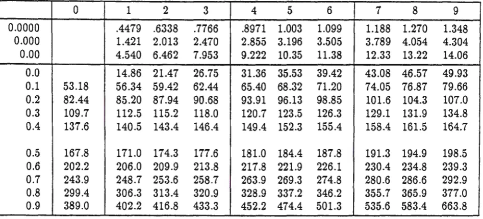
Table shewing values of <T for given

o

I

0 1 2 3 4 5 6 7 8 9

0.0000 .4479 .6338 .7766 .8971 1.003 1.099 1.188 1.270 1.348

0.000 1.421 2.013 2.470 2.855 3.196 3.505 3.789 4.054 4.304

0.00 4.540 6.462 7.953 9.222 10.35 11.38 12.33 13.22 14.06

0.0 14.86 21.47 26.75 31.36 35.53 39.42 43.08 46.57 49.93

0.1 53.18 56.34 59.42 62.44 65.40 68.32 71.20 74.05 76.87 79.66

0.2 82.44 85.20 87.94 90.68 93.91 96.13 98.85 101.6 104.3 107.0

0.3 109.7 112.5 115.2 118.0 120.7 123.5 126.3 129.1 131.9 134.8

0.4 137.6 140.5 143.4 146.4 149.4 152.3 155.4 158.4 161.5 164.7

0.5 I

167.8 I

171.0 174.3 177.6 181.0 184.4 187.8 191.3 194.9 198.5

I

0.6 202.2 206.0 209.9 213.8 217.8 221.9 226.1 230.4 234.8 239.3

0.7 243.9 248.7 253.6 258.7 263.9 269.3 274.8 280.6 286.6 292.9

I

0.8 299.4 306.3 313.4 320.9 328.9 346.2 '

355.7 377.0

337.2 365.9

0.9 389.0 402.2 416.8 433.3 452.2 474.4 501.3 535.6 583.4 663.8

(For values of 8 between 0.1 and 0.6 the expression <T

=

3008

+

20 gives an approximation to within a

few percent.)

An example

Suppose a machine has probability of failure 1/100 in any one day. So that p

=

1/100, and the MTTF

is 100 days. Suppose the profit per day is $1000, so that a

=

1000, and the expected profit before failure

is $100 000. If the cost of repair b

=

$5000 and the cost of each inspection c

=

$100, expressing these as percentages of $100000 (= a/p), we have f3

=

5 and 1

=

0.1.

Thus 8

=

0.1/95

=

1.05 x 10-3_{. Interpolation in the table, or numerical solution for this 6, gives}

<T

=

4.66. So the optimum period between inspections is 4.66% of the MTTF, that is 4.66 days. Substituting

these values in (1) gives the maximum value of the expected profit per unit time z

=

$906 per day. By comparison, inspection every day gives z

=

$845, and inspection every 10 days gives z

=

$894.

Discussion

It is of interest to consider the following diagram, which plots lines of equal 5 (which are therefore also lines of equal o-) against axes representing {3 and

r:

·

The contours a.re straight lines, since for any constant 5 we have

r

=

5(100 - {3), from (5). From the diagram we can 5ee that if the relative cost of inspection goes up-that is if

r

increases-with all the other parameters remaining the same, then the optimum period between inspections also lengthens, as we should expect. However, it also turns out that the inspection period should lengthen if the relative cost of repair goes up. This may seem rather paradoxical. Evidently in such circumstances it pays to gamble on the machine working for a bit longer than expected.

The line {3

+

r =

100 corresponds to the relation b

+

c

=

a/p, the expected profit before failure. So it represents the dividing line between profit and loss.

It is worth noticing that if;, the relative cost of inspection, gets high, in fa.ct if;

>

26.5, then the best inspection period is actually greater than the MTTF. As a fairly extreme case suppose that in our original example (with p

=

1/100) the cost of inspection is $90 000. We have ;

=

90, {3

=

5, 5

=

0.947 giving

o-

=

468. Thus the best inspection period is 468 days! Such circumstances might a.rise in, say, gravity-free manufacture in a satellite, when inspection costs could be very high.

Aknowledgment

I thank my colleague Dr P. Cerone for interesting me in this problem.

References

[l] A.H-S.Ang and W.H.Tang, Probability Concepts

in

Engineering Planning and Design, vol 2, Wiley, N.Y.,(1984].

[2] D.M.Brender, A surveillance model for recurrent events, IBM Reseach Report RC-837, Yorktown Heights, N .Y.,[1962].

(3] A.S.Goldman and T.B.Slattery, Maintainability: A Major Element of System Effectiveness, Krieger,

Hunt-ington, N.Y.,(1977].

[4] A.K.S.Jardine, Maintenace, Replacement, and Reliability, Pitman, London,[1973].

[5] M.Kamins, Determining Checkout Intervals for Systems Subject to Random Failures, RAND Corporation,

RM-2578, Santa Monica, Ca.,(1960]. ·

M.J .C.Baker,

Department of Mathematics, Computing and Operations Research, Footscray Institute of Technology