Article
1
Trace gas retrieval from AIUS
:
Algorithm description
2
and O
3retrieval assessment
3
Xiaoying Li1, Tianhai Cheng1,* Jian Xu2,*, Hailiang Shi3, Xingying Zhang4, Shule Ge5,
4
Mingmin Zou1, Hongmei Wang1, Yapeng Wang1, Songyan Zhu1 and Jing Miao1
5
1. State Key Laboratory of Remote Sensing Science, Institute of Remote Sensing and Digital Earth, Chinese
6
Academy of Sciences, Beijing 100101, China; [email protected] (X.L.)
7
2. Remote Sensing Technology Institute, German Aerospace Center (DLR), Oberpfaffenhofen, Germany
8
3. Anhui Institute of Optics and Fine Mechanics, Chinese Academy of Sciences, Hefei, Anhui, 230031, China
9
4. National Satellite Meteorological Center China Meteorological Administration ,
10
5. China Center for Resources Satellite Data and Application, China
11
* Correspondence:[email protected] (T.C.), [email protected] (J.X.)
12
13
Abstract: AIUS (Atmospheric Infrared Ultraspectral Sounder) is an infrared occultation
14
spectrometer onboard the Chinese GaoFen-5 satellite, which covers a spectral range of 2.4--13.3 μm
15
(750--4100 cm-1) with a spectral resolution of about 0.02 cm-1. AIUS is designed to measure and
16
study chemical processes of ozone (O3) and other trace gases in the upper troposphere and
17
stratosphere around Antarctic. In this study, the corresponding retrieval methodology is described.
18
The retrieval simulations based on the simulated spectra of AIUS have been carried out, with a
19
focus on O3. The relative difference between the retrieved and the true O3 profiles is within 5% from
20
the 15km to 70km and about 10% below 15km. The corresponding averaging kernels illustrate that
21
the overall retrieval information mainly come from the spectra, not the a priori. The retrieval
22
experiments also demonstrate that the shape of the retrieved profiles resembles the shape of the
23
true profile even if the shape of the a priori profile is different from that of the true profile. Further,
24
we perform the O3 retrieval from the real ACE-FTS (Atmospheric Chemistry Experiment-Fourier
25
Transform Spectrometer) measurements and compare the results with the official ACE-FTS Level-2
26
products. Overall, both profiles agree well in the stratosphere where the retrieval sensitivity is
27
high. The relative difference between both profiles is about 15% below 70km, which may due to the
28
measurement errors and different forward model parameters.
29
Keywords: AIUS; Occultation; Retrieval algorithm; Microwindows; Ozone
30
31
1. Introduction
32
The annual occurrence of the Antarctic ozone hole has been well documented. For studying
33
ozone recovery, many efforts have been made to understand the chemical and dynamical processes
34
around Antarctic [1-3]. Occultation and limb sounding techniques have provided an important way
35
for remotely observing Earth’s middle atmosphere. These measurements have greatly promoted our
36
understanding of the chemical process of atmospheric composition in the upper troposphere and
37
stratosphere by providing profiles measurments with different altitudes. As compared to
38
nadir-viewing measurements, occultation/limb sounding measurements have higher vertical
39
resolution, which can be used to derive vertical information of atmospheric components.
40
Furthermore, high-resolution atmospheric mid-infrared spectra are suitable for detection of many
41
trace species, since a wide variety of vibrational-rotational bands with molecular absorption lines are
42
found within this spectral range. Recently, many occultation observation/limb sounding sensors
43
have been developed and provided abundant profiles of trace gases, such as O3, CO, H2O, NO, etc
44
[4-9].
45
AIUS is one of six payloads onboard the Chinese GaoFen-5 satellite that is expected to launch in
46
May, 2018. AIUS is the first occultation spectrometer developed in China, which is designed to
47
detect the trace gases over the Antarctic. AIUS will operate in a solar synchronous orbit, with a
48
nominal height of 700 km. The instrument is a Fourier transform infrared spectrometer and its main
49
objective is to measure the O3 and other species in the stratosphere and upper troposphere in order
50
to study the ozone change over the Antarctic.
51
The aim of this study is to introduce the trace gas retrieval algorithm developed for AIUS and to
52
assess its performance based on ozone retrievals. In Section 2, the instrument parameters and level 1
53
processing of AIUS are introduced briefly. Section 3 describes the retrieval algorithm in detail.
54
Integrated atmosphere profiles dataset is presented and a sensitivity analysis of atmosphere profiles
55
is showed in Section 4. In Section 5, the simulated spectra and the ACE-FTS observation spectra are
56
adopted to retrieve O3 profiles and to assess the retrieval performance.
57
2. AIUS instrument
58
AIUS is a Fourier transform infrared spectrometer for the detection of occultation transmittance
59
spectra in the middle and upper atmosphere, which has similar characteristics to ACE-FTS. Both
60
instruments have a spectral resolution of 0.02 cm-1. AIUS covers the spectral range from 750 cm-1 to
61
4100 cm-1, while ACE-FTS covers 750--4400 cm-1. It is a dual-band system composed of MCT
62
(mercury cadmium telluride, 750--1850 cm-1) and InSb (1850--4160 cm-1). AIUS covers an altitude
63
range from 8 to 100 km and has a field of view of 1.25 mrad. The latitude coverage of AIUS
64
measurements is about 55°S to 90°S, which is mostly over Antarctica.
65
GF5-AIUS level 0 is original auxiliary and interferogram data in binary format and level 1 is
66
HDF5 format file includes reconstructed spectra and processed auxiliary data. GF5-AIUS level 0 to
67
level 1 processing includes three steps. The first step is the acquisition and processing of auxiliary
68
data. By unpacketizing the auxiliary data package, the information of observation, such as
69
acquisition time, sun position and satellite position, is acquired. The geometric parameters, the
70
height and the latitude and longitude coordinates, are calculated from the information of the sun
71
and satellite. The second step is to reconstruct the spectra from the original interferogram. However,
72
since the AIUS is an interferometer, the interferogram will contain some spikes produced by the
73
effect of energetic particles due to space electromagnetic environment on orbit, which will
74
contaminate the complete spectra. Thus, some processes have to be involved to correct these errors.
75
The nonlinear behavior of the detectors is expected and characterized on-ground, which requires an
76
additional correction. This nonlinearity correction will be consolidated in-flight using
77
commissioning phase data. After that, the FFT is performed to compute the spectra. The last step is
78
to evaluate the spectra’s quality by standard deviation or mean value of imaginary part of the
79
calculated spectra and then make the mark to show if the spectra is well reconstructed. “0” is for
80
good quality and “1” for bad quality.
81
Level 1 data is the spectra data which are the relative intensities of each tangent heights using
82
DN (digital number) values. Our inversion takes the transmittance converted from the Level 1 data.
83
In addition to the observation of the Sun outside and inside the atmosphere, GF5-AIUS also observes
84
the deep space to remove the instrumental emission. Commonly, the transmittance (ℎ, ) at
85
tangent point h of wave number can be calculated by the following equation:
86
(ℎ, ) =
( , ) ( )( ) ( )
, (1)
87
Where (ℎ, ), ( ) and ( ) are the digital counts of the observation of signal at tangent point h,
88
the solar radiation outside atmosphere and the deep space signal.
89
3. Retrieval methodology of AIUS
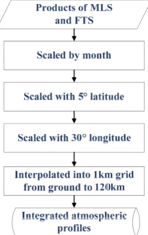
90
Accurate knowledge of pointing and p/T information is important to high-precision
91
quantitative retrieval of abundances of atmospheric species from occultation observed
92
transmittances. The tangent height correction for AIUS is carried out by employing the triangular
iteration with tangential strides technique in a microwindow of N2 continuum absorption, whereas
94
the scheme of p/T retrieval is by introducing the hydrostatic equation into the iterative process of
95
optimal algorithm. Details of the design and development of these two algorithms are introduced in
96
our other two papers in preparation.
97
3.1. Inversion model
98
The inversion algorithm employed in this study is based on OEM (Optimal Estimation
99
Method) proposed by Rodgers [10]. Since OEM is generally applicable and facilitates a theoretical
100
error analysis, this method has been widely used in the inversion of atmospheric state parameters
101
using infrared and microwave remote sensing measurements, with nadir, occultation or limb
102
viewing [11-16]. OEM stabilizes the inversion process by taking into account the statistical
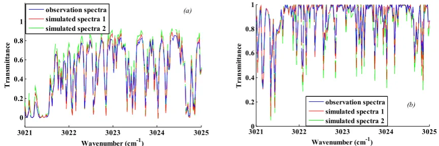
103
information about the atmospheric variability, which has been investigated by many studies
104
[17-23].
105
Our inversion scheme is adapted from the retrieval software Qpack 2.0 [23] that uses LM
106
(Levenberg—Marquardt) approach for a nonlinear least squares fitting. The LM iteration method
107
adopted in the Qpack is the same as the LM iteration method modified by Rodgers [17]. By
108
introducing a constraint factor γ, the next iterate is yielded by:
109
=
+ [(1 + )
+
∙
∙
]
∙
[ − ( )] −
[
−
] .
(2)
110
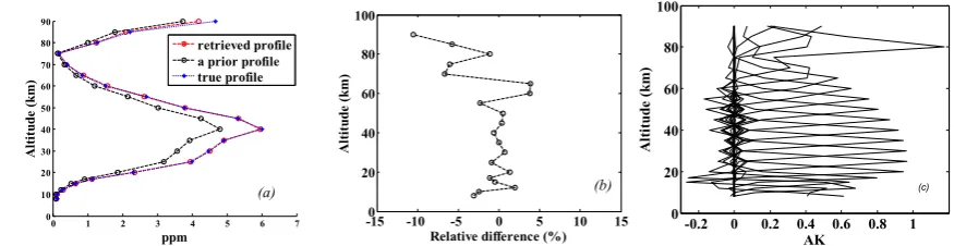
The inverse of the solution covariance in equation (2) is given by
:
111
=
∙
∙
. (3)
112
113
And the cost function ( ) is given by:
114
( ) = [
− ( ) ∙
∙
− ( ) + ( −
) ∙
∙ ( −
)]/
, (4)
115
where is the forward model, is a series of observations value, is the state of the
116
atmosphere, is the covariance matrix of the observation error and is the matrix of weighting
117
function. The a priori state vector is denoted by , with its covariance matrix And is the
118
number of vector.
119
In our retrieval scheme, retrieval experiments are made based on many simulated spectra and
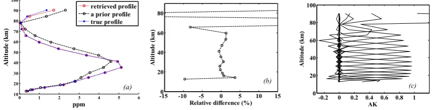
120
ACE-FTS observation data to decide an optimal choice of γ. After statistical analysis, the factor of γ
121
is defined as a linear scaled function to the cost function. It will be updated at each iteration, which
122
is given by the following equation. Here, is a constant and it is different for different
123
atmospheric species.
124
γ = ∙ ( )
. (5)
125
The definition of the a priori covariance matrix
follows Gaussian statistics and
126
considers the correlation
betweendifferent components of the state vector and the forward
127
model vector. Different types of the correlation function [24] for computing the correlation
128
have been tested based on the retrievals from simulated and observed ACE-FTS data. In
129
this study, we employ the linear correlation function:
130
( , ) = max 0, ( ) ( ) 1 − (1 −
)
| ( )( ) ( )|( ), (6)
131
where i and j are position indexes, z is the position, lc is the correlation length and |*| signifies the
132
absolute value.
σ
is the standard deviation calculated from the a priori.133
In the retrieval scheme of AIUS, we adopt the “ ” in the Qpack 2.0 as the threshold of
134
convergence. The iteration is considered converged in the condition that the value of is smaller
135
than 0.01. The definition of is that:
136
= [(
−
) ∙
∙ (
−
)]/
, (7)
137
where is the length of the state vector.
3.2 Adopted forward model
139
An accurate modeling of the radiative transfer through the atmosphere plays an important role
140
in the inversion. The forward model adopted in the retrieval algorithm of AIUS is the RFM
141
(Reference Forward Model) with the latest release version v4.36 [25]. RFM is a GENLN2-based
142
line-by-line radiative transfer model originally developed at AOPP, Oxford University, under an
143
ESA contract to provide reference spectral calculations for the MIPAS (The Michelson Interferometer
144
for Passive Atmospheric Sounding) instrument launched on the ENVISAT (Environmental Satellite)
145
in 2002. It has been subsequently developed into a general purpose code suitable for a variety of
146
different spectroscopic calculations. Von Clarmann [26] has compared five forward models
147
including the RFM. The inter-comparison experiment showed that the overall inter-consistency of
148
spectra for all participants is good, which also can demonstrate that the RFM works fine and reliable.
149
RFM can deal with various measurement conditions including nadir viewing, limb sounding,
150
occultation observation from different platforms (satellite /balloon /aircraft). Its main features are
151
listed below:
152
1. It has high flexibility when defining observation geometry (including scanning features) and
153
sensor characteristics.
154
2. It can provide Jacobians for p, T, VMR, line-of-sight pointing and surface temperature and
155
emissivity.
156
3. Cross sections can be computed from HITRAN (High-resolution Transmission) spectroscopic
157
database or read from external files.
158
4. Continua for H2O, O2, N2 and CO2 are included [27-31].
159
For all considered microwidows, scattering can be negligible and is not taken into accout in our
160
retrieval scheme.
161
3.3 Microwindows
162
The spectral resolution of AIUS is about 0.02 cm-1. Because of this, the number of data points
163
from each absorption band becomes unrealistic for an efficient inversion process. Furthermore, one
164
should avoid the effect of interfering species on the retrieval of the target species and have the best
165
information on the retrieval. Thus, the retrieval is performed using a set of narrow spectral interval
166
(called "microwindow") instead of an entire spectral band.
167
To select an appropriate set of microwindows, a sensitivity analysis with Jacobians is required.
168
First of all, we select the spectral points which are sensitive to the target gas on each cutting height
169
and are not sensitive to the interference gas according to the Jacobians of target and the interference
170
species. Then, the selected spectral points are grown on the basis of information entropy to generate
171
a series of continuous window. Finally, all the selected microwindows at different tangent height are
172
combined.
173
The absorption lines of O3 in the infrared band are mainly located near 9.6 μm and the main
174
interfering gases of O3 in this spectral band include CO2, H2O and N2O. The chosen microwindows
175
for O3 retrieval are shown in Figure 1. For O3 retrieval, about 20 microwindows are selected, covering
176
from 5 km to 95 km. Microwindows in the range of 1000--1070 cm-1 are sensitive at higher altitudes,
177
while others are sensitive at lower altitudes.
179
Figure 1 The microwindows selected for O3 retrieval.
180
4. Sensitivity analysis of atmospheric profiles in forward model
181
4.1 Integrated Atmospheric profiles
182
The forward model generates a numerical simulation of measurements based on the given
183
atmospheric state. In other words, the accuracy of the simulated measurements depends on the
184
reliability of the atmospheric parameters used in the forward model. In our retrieval scheme, we
185
compute a dataset of integrated atmospheric profiles based on MLS (Microwave Limb Sounder)
186
level 2 products, ACE-FTS level 2 products and the profiles from AFGL(Air Force Geophysics
187
Laboratory) atmospheric models.
188
The ACE-FTS level 2 v3.6 and the MLS level 2 (v4.2) products between 2014 and 2016 are
189
considered. We classify and store the species profiles month by month for each set of products. Then,
190
the monthly mean profiles are acquired and classified into different coordinate grids, which is
191
discretized with a 5° latitude and 30° longitude spacing.. That is, both of two set of dataset are
192
classified by month and coordinate grid. A diagram of constructing the integrated atmospheric
193
profiles is shown in Figure 2.
194
195
Figure 2 The technological process of constructing the integrated atmospheric profiles.
The next step is to combine the two sets of profiles. Since ACE-FTS and AIUS have similar
197
instrument characteristics, the ACE-FTS product is chosen in case that the profile of a particular
198
species at the same geolocation and time can be found in both ACE-FTS and MLS datasets. Finally,
199
profiles of the missing species are read from the AFGL dataset. The species profiles imported from
200
AFGL dataset include NH3, HBr, HI, PH3, H2S, F11, F12, F13, F21, F22, F114, F115 and HNO4. These
201
species profiles from FASCOD (Fast Atmospheric Signature Code) Model 1-6 are resampled and
202
packed into the monthly geographic grids. In the end, the integrated atmospheric species profiles
203
dataset is produced.
204
4.2 Data simulation and sensitivity analysis
205
A comparison between the integrated atmospheric and AFGL profiles is carried out by
206
simulating the ACE-FTS spectra. The simulation is made with the geolocation and geometry
207
parameters of the ACE-FTS instrument. Figures 3 and 4 compare the simulated ACE-FTS using the
208
two atmospheric profiles database to the observed spectra in two spectra ranges.
209
Figure 3 Comparison experiment between the integrated atmospheric and AFGL profiles (67.5°S,
210
72.5°W, August 5, 2012). (a) Tangent height=10.71 km; (b) Tangent height=20.48 km.
211
Figure 4 Comparison experiment between the integrated atmospheric and AFGL profiles (77°S, 86°E,
212
March 25, 2012). (a) Tangent height=16.16 km; (b) Tangent height=30.4 km.
213
214
The simulated spectra 1 and 2 stand for the ones using the integrated atmospheric and AFGL
215
profiles, respectively. Figures 3 and 4 show that in both spectral ranges, the simulated spectra using
216
the integrated atmospheric profiles are obviously more close to the ACE-FTS observed spectra than
217
those using the AFGL atmospheric profiles. The two comparison experiments demonstrate that the
218
simulated spectra are very sensitive to the atmospheric profiles and that the simulated spectra using
219
the dataset of integrated atmospheric profiles agree well to the actual measurements.
220
221
222
1311 1312 1313 1314 1315
0 0.1 0.2 0.3 0.4 0.5
Tr
an
sm
it
ta
nc
e
Wavenumber (cm-1)
observation spectra simulated spectra 1 simulated spectra 2
(a)
1311 1312 1313 1314 1315
0 0.2 0.4 0.6 0.8 1
T
ra
n
sm
itta
n
ce
Wavenumber (cm-1)
simulated spectra 2 simulated spectra 1 observation spectra
(b)
3021 3022 3023 3024 3025
0 0.2 0.4 0.6 0.8 1
T
ra
n
sm
itta
n
ce
Wavenumber (cm-1)
observation spectra simulated spectra 1 simulated spectra 2
(a)
30210 3022 3023 3024 3025
0.2 0.4 0.6 0.8 1
T
ra
n
sm
itta
n
ce
Wavenumber (cm-1)
observation spectra simulated spectra 1 simulated spectra 2
5. O3 retrieval and assessment
223
5.1 Assessment of retrieval algorithm based on simulated spectra
224
Table 1 Retrieval configuration
225
Parameters Retrieval configuration
spectroscopic database Hitran 2012 [32]
continua used O2, H2O, N2
Retrieval altitude grids /km 8 10 12 15 17 20 25 30 35 40 45 50 55 60 65 70
75 80 85 90
altitude grids in the forward model 0-100 km with 1 km resolution
O3 true profiles (X_true) Taken from integrated atmospheric
database
0.8 ∙ _
226
The O3 retrieval performance is first assessed by using simulated measurements. The
227
microwindows selected in section 3.3 are adopted. Two O3 profiles picked from two grids of the
228
integrated atmospheric dataset (75°S, 150°W in October and 65°S, 90°E in March) are taken as the
229
true profiles to simulate spectra of AIUS. Then, the artificial noise with SNR = 300 is added to the
230
simulated spectra. Details of retrieval configuration are specified in Table 1. The retrieved profiles
231
are shown in Figure 5 and 6.
232
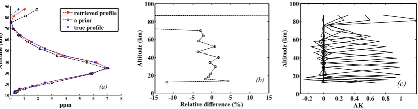
233
Figure 5 O3 retrieval experiment based on simulated spectra at 75°S, 150°W in October. (a)Retrieved
234
profile; (b) Relative difference between retrieved and true profiles; (c) Averaging kernel.
235
236
Figure 6 O3 retrieval experiment based on simulated spectra at 65°S, 90°E in March. (a)Retrieved profile;
237
(b) Relative difference between retrieved and true profile; (c) Averaging kernel.
238
239
The a priori, true profile and retrieval profile of O3 are shown in figure 5(a) and 6(a). The shape
240
and the values of retrieval profiles are consistent with the true profiles. The relative difference
241
between the retrieval and true profiles presented in figure 5(b) and 6(b) shows that it is within ±5%
242
below 60 km, within ±7% from 60 km to 80 km. The averaging kernels in figure 5(c) and 6(c) illustrate
243
that the retrieval information mainly comes from the measurements.
244
0 2 4 6 8
0 20 40 60 80 100
ppm
Al
ti
tude
(
km
)
retrieved profile a prior profile true profile
(a)
-150 -10 -5 0 5 10 15
20 40 60 80 100
A
lt
it
ude
(
km
)
Relative difference (%)
(b)
-0.20 0 0.2 0.4 0.6 0.8 1
20 40 60 80 100
AK
Al
ti
tude
(
km
)
(c)
0 1 2 3 4 5 6 7 0
10 20 30 40 50 60 70 80 90
ppm
Al
ti
tude
(
km
)
retrieved profile a prior profile true profile
(a)
-150 -10 -5 0 5 10 15
20 40 60 80 100
Al
ti
tude
(
km
)
Relative difference (%)
(b)
-0.2 0 0.2 0.4 0.6 0.8 1
0 20 40 60 80 100
AK
Al
ti
tude
(
km
)
As the residual in both experiments seems nearly identical, only the one in the first experiment
245
is shown in Figure 7.The lowest to the highest tangent heights is from left to right. The residuals at
246
each tangent height are within ±0.02, which are very small.
247
248
Figure 7 The residuals of the first retrieval experiment.
249
In the above retrieval experiments, = 0.8 ∙ _ , but the shape is same. Thus, more
250
retrieval experiments are made to assessment the dependence of the AIUS algorithm on the shape of
251
the a prior profile. In this experiment, the ACE-FTS O3 level 2 products are taken as the true profiles.
252
The information of five products selected is shown in table 2. The a prior profiles are from the mean
253
monthly profiles of MLS O3 level 2 products, which indicates that the shape of the a prior profiles
254
can be different from that of the true profiles.
255
Table 2 Information of O3 L2 products from ACE-FTS.
256
Scene ID latitude longitude date
40993 -78 87 2012-3-25
39926 -68 131 2011-1-11
38154 63 -73 2010-9-13
43544 63 75 2011-9-14
43611 70 -119 2011-9-18
Similarly, the artificial noise with same SNR is added randomly to the simulated spectra. O3
257
retrieval is performed and the results for these five retrieval experiments are similar. Thus, only
258
results of two retrieval experiments using the O3 products from scenes of 40993 and 38154 are
259
presented in Figures 8 and 9, respectively. The two scenes are located in Antarctica and Arctic,
260
respectively.
261
262
Figure 8 O3 retrieval experiment based on O3 product from scene 40993 of ACE-FTS. (a)Retrieved profile;
263
(b) Relative difference between retrieved and true profile; (c) Averaging kernel.
264
0 1 2 3 4 5 6 7 8 9 10 11 12 13 14 15 16 16 18 19 20 -0.02
-0.01 0 0.01 0.02
Number of tangent heights
R
es
id
ua
ls
(
Y-Yf
)
0 1 2 3 4 5 6 10
20 30 40 50 60 70 80 90 100
ppm
Al
ti
tu
de
(
km
)
retrieved profile a prior profile true profile
(a)
-150 -10 -5 0 5 10 15
20 40 60 80
A
lti
tu
de
(
km
)
Relative difference (%)
(b)
-0.2 0 0.2 0.4 0.6 0.8 1 0
20 40 60 80 100
AK
A
lt
it
ude
(
km
)
265
Figure 9 O3 retrieval experiment based on O3 product from scene 38154 of ACE-FTS. (a)Retrieved profile;
266
(b) Relative difference between retrieved and true profile; (c) Averaging kernel.
267
268
Figures 8(a) and 9(a) show that the shape of the retrieval profiles is almost the same with the
269
true profiles even that the shape of the a prior profiles is different from that of the true profiles.
270
Figures 8(b) and 9(b) illustrate that the relative difference between the retrieval O3 profiles and the
271
true O3 profiles is almost within 5% from 10 km to 70 km, about 10% near 10 km. However, the
272
relative difference will reach beyond 30%. The reasons may be due to the low concentration of O3
273
profiles and the retrieval above 70 km is dominated by the a priori information The averaging
274
kernels in Figures 8(c) and 9(c) are similar as those in Figures 5(c) and 6(c), which indicate that the
275
retrieval information mainly comes from the measurement in the troposphere and stratosphere. We
276
also check the residuals of these five retrieval experiments, which are consistent with the residuals in
277
Figure 7. All residuals of these five retrieval experiments are within ±0.02.
278
The retrieval experiments using synthetic AIUS spectra demonstrate that the algorithm
279
produces reasonable results and sufficient retrieval sensitivity.
280
5.2 O3 retrieval based on ACE-FTS measurements
281
Under real-world conditions, in addition to the thermal noise of the instrument, the actual
282
measurements are influenced by more factors. To evaluate the influence of various uncertainties on
283
the retrieval algorithm of AIUS, we adopt the level 1 products of ACE-FTS to perform the O3
284
retrieval experiments, as AIUS expects to perform measurements with similar characteristics. All the
285
a prior profiles of O3 and other species are taken from the dataset of integrated atmospheric profiles.
286
The level 1products used are those five scenes of ACE-FTS observation data in table 2. Since the
287
results for these five retrieval experiments are similar, only results of two retrieval experiments from
288
scene 40993 and 38154 are presented.
289
290
291
Figure 10 O3 retrieval experiment based on FTS observation spectra from scene 40993. (a)Retrieved profile;
292
(b) Relative difference between retrieved and FTS level 2 product; (c) Averaging kernel.
293
294
0 1 2 3 4 5 6 7 8 10 20 30 40 50 60 70 80 90 ppm A lti tu de ( km ) retrieved profile a prior true profile (a)
-150 -10 -5 0 5 10 15
20 40 60 80 100 A lti tu de (k m )
Relative difference (%)
(b)
-0.2 0 0.2 0.4 0.6 0.8 1
0 20 40 60 80 100 AK A ltitu de ( km ) (c)
0 2 4 6
0 20 40 60 80 100 ppm A ltit ud e (k m) retrieved profile ACE-FTS profuct (a)
-30 -20 -10 0 10 20 30
0 20 40 60 80 100 A lt it ude ( km )
Relative difference (%)
(b)
-0.20 0 0.2 0.4 0.6 0.8 1
295
Figure 11 O3 retrieval experiment based on FTS observation spectra from scene 38154. (a)Retrieved profile;
296
(b) Relative difference between retrieved and FTS level 2 product; (c) Averaging kernel.
297
298
The retrieval profiles, the relative difference and averaging kernels are shown in figure 10 and
299
11. The retrieval profiles presented in figure 10(a) and 11(a) show that the shape of the retrieval O3
300
profiles agree well to those of ACE-FTS level 2 products. However, the relative difference in figure
301
10(b) and 11(b) is bigger than that in figure 8(b) and 9(b). The relative difference of these two
302
retrieval experiment below 70 km is mainly within 10%, with some points reach 15%-20%. The
303
relative difference here is larger mainly because of the uncertainties in the measurements and
304
different forward model parameters. The bias of the ACE-FTS O3 products is +1 to +8% in the
305
stratosphere (16–44 km) and can be up to +40% (+20% on average) above 45 km (Jones A., et al., 2012;
306
Dupuy E., et al., 2009). Although the averaging kernels in Figures 10(c) and 11(c) are somewhat
307
broader than those in Figures 8(c) and 9(c), it still reveals that the retrieval information mainly comes
308
from the measurement in the stratosphere. The statistical analysis of the residuals demonstrate that
309
about 90% residuals are within ±0.02, with some points reaching ±0.06, demonstrating the retrieval
310
fits very well. Our algorithm dedicated to AIUS performs stable and delivers comparable results
311
using ACE-FTS real measurements.
312
6. Discussion and conclusions
313
In this study, we have introduced a retrieval algorithm developed for an infrared occultation
314
spectrometer called AIUS. The retrieval algorithm comprises a forward model based on RFM and
315
an OEM framework adapted from Qpack, which employs the LM iteration method. The retrieval
316
experiments of ozone retrievals were carried out based on simulated spectra and ACE-FTS
317
measurements.
318
In the condition of experiments on simulated spectra, there are some differences depending
319
on the profile shape of the a prior. When the shape of the a prior is the same as the true profile, the
320
relative difference between the retrieval profile and the true profile is within ±5% below 60 km and
321
within 7% in the range of 60-80 km. When the shape of the a prior is and the true profile is different,
322
the retrieval profile shape still keep close to the true profile. The relative difference is a litter bigger.
323
It is mainly within 5% below 60 km, but can reach 10% near 10 km and 10-15% from 60 km to 70 km.
324
However, the relative difference is in a reasonable range. And the averaging kernels achieved
325
illustrate that the retrieval information mainly comes from the simulated observation spectra. Thus
326
the retrieval experiments based on simulated spectra indicate that the retrieval algorithm of AIUS
327
work fine and successful.
328
When it comes to experiments based on ACE-FTS observation data, the retrieval algorithm of
329
AIUS also behaves well. The retrieval experiments show that the relative differences between them
330
are greater than those in the retrieval experiments using simulated spectra. The greater relative
331
differences may be produced by the following reasons. Firstly, although the instrument parameters
332
AIUS and FTS are similar, there must be different in some of the details. Thus, some errors will be
333
brought by using ACE-FTS observation spectra as the AIUS observation spectra. Secondly, the
334
ACE-FTS levels are not the true profiles. They also have uncertainties, which will make the relative
335
difference greater. The last and the most important reason is the greater uncertainty of the observed
336
spectra, which will generate some errors between the simulated spectra by the forward model and
337
0 2 4 6 8 10
20 30 40 50 60 70 80 90
ppm
A
lti
tu
de
(k
m
)
retrieved profile ACE-FTS product
(a)
-30 -20 -10 0 10 20 30
0 20 40 60 80 100
A
lti
tu
de
(k
m
)
Relative difference (%) (b)
-0.20 0 0.2 0.4 0.6 0.8 1
20 40 60 80 100
AK
Al
ti
tu
de
(
km)
the observation spectra in the retrieval process. Nevertheless, the retrieval profiles still agree well
338
with the ACE-FTS level 2 products and the range of the relative differences is satisfactory.
339
All the retrieval experiments based on the simulated spectra and the measured spectra of
340
ACE-FTS indicate that the retrieval algorithm of AIUS is reliable and robust. Overall, the retrieval
341
profiles agree well with the true profiles or the ACE-FTS level 2 profiles. However, the uncertainties
342
of the retrieval profiles at lower tangent height are still requiring further investigations. After the
343
instrument is launched, we will improve the retrieval algorithm by fine-tuning the forward model
344
parameters according to the characteristics of the AIUS observed spectra and the instrument
345
performance. In addition, an extensive retrieval error characterization is on-going and will be
346
consolidated during the operational phase.
347
348
349
Acknowledgments: This study was supported in part by the project 41571345 supported by National Natural
350
Science Foundation of China, the National Key Research and Development Program of China (Grant No.
351
2016YFB0500705), the project supported by the Special Foundation for Free Exploration of State Laboratory of
352
Remote Sensing Science (Grant No. Y1Y00202KZ), and the project supported by Major Projects of High
353
Resolution Earth Observation System (Grant No. 32-Y20A18-9001-15-17-1). The ACE-FTS data were provided
354
by ACE-FTS team. ACE, also known as SCISAT, is a Canadian-led mission mainly supported by the Canadian
355
Space Agency (CSA). And Thanks to Professor Anu Dudhia for providing the RFM source code and help.
356
Author Contributions: Xiaoying Li, Tianhai Cheng and Jian Xu conceived and designed the experiments;
357
Mingmin Zou, Hongmei Wang, Yapeng Wang, Songyan Zhu and Jing Miao performed the experiments;
358
Xiaoying Li, Tianhai Cheng, Jian Xu, Hailiang Shi, Xingying Zhang andShule Ge analyzed the data; Xiaoying
359
Li wrote the paper.
References
362
1. Manney, G.L.; Santee, M.L.; Livesey, N.J.; Froidevaux, L.; Read, W.G.; Pumphrey, H.C.; Waters, J.W.;
363
Pawson, S. EOS Microwave Limb Sounder observation of the Antarctic polar vortex breakup in 2004.
364
Geophysical Research Letters. 2005, 32(L12811), 1-5, DOI: 10.1029/2005GL022823.
365
2. Santee, M.L.; Manney, G.L.; Livesey, N.J.; Froidevaux, L.; MacKenzie, I.A.; Pumphrey, H.C.; Read, W.G.;
366
Schwartz, M.J.; Waters, J.W.; Harwood, R.S. Polar processing and development of the 2004 Antarctic
367
ozone hole: First results from MLS on Aura. Geophysical Research Letters. 2005, 32(L12817), 1-4, DOI:
368
10.1029/2005GL022582.
369
3. Gattinger, R. L.; McDade, I. C.; Alfaro Suzan, A. L. ; Boone, C. D.; Walker, K.A.; Bernath, P.F.; Evans, W.F.
370
J.; Degenstein, D.A.; Yee, J.-H.; Sheese, P.; Llewellyn, E. NO2 air afterglow and O and NO densities from
371
Odin-OSIRIS night and ACE-FTS sunset observations in the Antarctic MLT region. Journal of Geophysical
372
Research. 2010, 115 (D12) , 1256-1268, DOI: 115. 10.1029/2009JD013205.
373
4. Russell, J.M.; Gordley, L.L.; Park, J.H.; Drayson, S.R.; Hesketh, W.D.; Cicerone, R.J.; Tuck, A.F.; Frederick,
374
J.E.; Harries, J.E.; Crutzen, P.J. The Halogen Occultation Experiment. Journal of Geophysical
375
Research-Atmospheres. 1993, 98(D6), 10777-97.
376
5. Gunson, M.R.; Abbas, M.M.; Abrams, M.C.; Allen, M.; Brown, L.R.; Brown, T.L.; Chang, A.Y.; Goldman,
377
A.; Irion, F.W.; Lowes, L.L.; Mahieu, E.; Manney, G.L.; Michelsen, H.A.; Newchurch, M.J.; Rinsland, C.P.;
378
Salawitch, R.J.; Stiller, G.P.; Toon, G.C.; Yung, Y.L.; Zander, R. The Atmospheric Trace Molecule
379
Spectroscopy (ATMOS) experiment: Deployment on the ATLAS Space Shuttle missions. Geophysical
380
Research Letters. 1996, 23(17), 2333-2336.
381
6. Bovensmann, H.; Burrows, J.P.; Buehwitz, M.; Frerick, J.; Noel, S.; Rozanov, V.V. SCIAMACHY: Mission
382
Objectives and Measurement Modes. Journal of the atmospheric sciences.1999, 56(2), 127-150.
383
7. Beer, R.; Glavich, T.A.; Rider, D.M. Tropospheric emission spectrometer for the Earth Observing System's
384
Aura Satellite. Applied Optics. 2001, 40(15), 2356-67.
385
8. Bernath P.F.; McElroy C.T.; Abrams M.C.; Boone, C.D.; Butler, M.; Camy-Peyret, C.; Carleer, M.; Clerbaux,
386
C.; Coheur, P.-F.; Colin, R.; DeCola, P.; DeMazie`re, M.; Drummond, J. R.; Dufour, D.; Evans, W. F. J.; Fast,
387
H.; Fussen, D.; Gilbert, K.; Jennings, D.E.; Llewellyn, E. J.; Lowe, R.P.; Mahieu, E.; McConnell, J.C.;
388
McHugh, M.; McLeod, S.D.; Michaud, R.; Midwinter, C.; Nassar, R.; Nichitiu, F.; Nowlan, C.; Rinsland,
389
C.P.; Rochon, Y.J.; Rowlands, N.; Semeniuk, K.; Simon, P.; Skelton, R.; Sloan, J.J.; Soucy, M.-A.; Strong, K.;
390
Tremblay, P.; Turnbull, D.; A. Walker, K. ; Walkty, I.;. Wardle, D.A; Wehrle, V.; Zander, R., Zou, J.
391
Atmospheric Chemistry Experiment (ACE): Mission overview. Geophysical Research Letters. 2005, 32,
392
L15S01, doi:10.1029/2005GL022386.
393
9. Fischer, H.; Birk, M.; Blom, C.; Carli, B.; Carlotti, M.; Clarmann, T.von; Delbouille, L.; Dudhia, A.; Ehhalt,
394
D.; Endemann, M.; Flaud, J.M.; Gessner, R.; Kleinert, A.; Koopman, R.; Langen, J.; Lopez-Puertas´, M.;
395
Mosner, P.; Nett, H.; Oelhaf, H.; Perron, G.; Remedios, J.; Ridolfi, M.; Stiller, G.; Zander, R.. MIPAS: an
396
instrument for atmospheric and climate research. Atmos Chem Phys. 2008, 8(8), 2151-88.
397
10. Rodgers, C.D. Retrieval of atmospheric temperature and composition from remote measurements of
398
thermal radiation. Reviews of Geophysics and Space Physics. 1976, 14(4), 609-624.
399
11. Urban, J.; Baron, P.; Lautie, N.; Schneider, N.; Dassas, K.; Ricaud, P.; de la Noë, J. Moliere (v5): a versatile
400
forward- and inversion model for the millimeter and sub-millimeter wavelength range. Journal of
401
Quantitative Spectroscopy and Radiative Transfer. 2004, 83(3/4), 529-554, DOI: 10.1016/S0022-4073(03)00104-3.
402
12. Boone, C.D.; Nassar, R.; Walker, K.A.; Rochon, Y.; McLeod, S.D.; Rinsland, C.P.; Bernath, P.F. Retrievals
403
for the atmospheric chemistry experiment Fourier-transform spectrometer. Applied Optics. 2005, 44(33),
404
7218-31.
405
13. Raspollini, P.; Belotti, C.; Burgess, A.; Carli1, B.; Carlotti, M.; Ceccherini, S.; Dinelli, B.M.; Dudhia, A.;
406
Flaud, J.-M.; Funke, B.; Hopfner, M.; Lopez-Puertas, M.; Payne, V.; Piccolo, C.J.; Remedios, J.; Ridolfi, M.;
407
Spang, R. MIPAS level 2 operational analysis. Atmos. Chem. Phys.2006, 6, 5605–5630.
408
14. Livesey, N.J.; Snyder, W.V.; Read, W.G.; Wagner, P. A. Retrieval Algorithms for the EOS Microwave Limb
409
Sounder (MLS). IEEE Transactions on Geoscience and Remote Sensing. 2006, 44(5), 1144-1155.
410
15. Bowman, K.W.; Rodgers, C.D.; Kulawik, S.S.; Worden, J.; Sarkissian, E.; Osterman, G.; Steck, T.; Lou, M.;
411
Eldering, A.; Shephard, M.; Worden, H.; Lampel, M.; Clough, S.; Brown, P.; Rinsland, C.; Gunson, M.;
412
Beer, R. Tropospheric Emission Spectrometer: Retrieval Method and Error Analysis. IEEE Transactions on
413
Geoscience and Remote Sensing.2006, 44(5), 1297-1307.
16. Takahashi, C.; Ochiai, S.; Suzuki, M. Operational retrieval algorithms for JEM/SMILES level 2 data
415
processing system. Journal of Quantitative Spectroscopy & Radiative Transfer. 2010, 111, 160–173.
416
17. Rodgers, C.D. Inverse Methods for Atmospheric Sounding: Theory and Practice, Series on Atmospheric Oceanic and
417
Planetary Physics-Vol. 2, World Scientific Publishing Co. Pte. Ltd: P O Box 128, Farrer Road, Singapore,
418
2000; pp. 92-93, ISBN: 981-02-2740-X.
419
18. Eriksson, P. Analysis and comparison of two linear regularization methods for passive atmospheric
420
observations. Journal of Geophysical Research. 2000, 105(D14), 18,157-18,167.
421
19. Doicu, A.; Schreier, F.; Hess, M. Iteratively regularized Gauss – Newton method for atmospheric remote
422
sensing. Computer Physics Communications. 2002, 148, 214–26.
423
20. Steck, T. Methods for determining regularization for atmospheric retrieval problems. Applied Optics. 2002,
424
41(9), 1788-1797.
425
21. Jiang, D.M.; Dong, C.H. A review of optimal algorithm for physical retrieval of atmospheric profile.
426
Advances in Earth Science. 2010, 25(2), 133-139.
427
22. Zou, M.M.; Chen, L.F.; Li, S.S.; Fan, M.; Tao, J.H.; Zhang, Y. An improved constraint method in optimal
428
estimation of CO2 from GOSAT SWIR observations. Science China Earth Sciences. 2016, DOI:
429
10.1007/s11430-015-0247-9.
430
23. Xu, J.; Schreier, F.; Doicu, A.; Trautmann, T. Assessment of Tikhonov-type regularization methods for
431
solving atmospheric inverse problems. Journal of Quantitative Spectroscopy & Radiative Transfer. 2016, 184,
432
274–286.
433
24. Eriksson, P.; Jimeneza, C.; Buehler, S.A. Qpack, a general tool for instrument simulation and retrieval
434
work. Journal of Quantitative Spectroscopy & Radiative Transfer. 2005, 91, 47-64.
435
25. REFERENCE FORWARD MODEL. Available online: http://eodg.atm.ox.ac.uk/RFM/index.html.
436
26. Von Clarmann, T..; Hopfner, M.; Funke, B.; Lopez-Puertas, M.; Dudhia, A.; Jay, V.; Schreier, F.; Ridolfi, M.;
437
Ceccherini, S.; Kerridge, B.J.; Reburn, J.; Siddans, R. Modelling of atmospheric mid-infrared radiative
438
transfer: the AMIL2DA algorithm intercomparison experiment. Journal of Quantitative Spectroscopy &
439
Radiative Transfer. 2003, 78, 381-407.
440
27. Clough, S.A.; Kneizys, F.X.; Davies, R.W. Line shape and the water vapor continuum. Atmos. Res. 1989,
441
23, 229-241, DOI: 10.1016/0169-8095(89)90020-3.
442
28. Mlawer, E.J.; Payne, V.H.; Moncet, J.-L.; Delamere, J.S.; Alvarado, M.J.; Tobin, D.C. Development and
443
recent evaluation of the MT-CKD model of continuum absorption. Philosophical Transactions of the
444
Royal Society A: Mathematical, Physical and Engineering Sciences. 2012, 370 (1968),. 2520-2556, DOI:
445
10.1098/rsta.2011.0295.
446
29. Thibault, F.; Menoux, V.; Le Doucen, R.; Rosenmann, L.; Hartmann, J.-M.; Boulet, Ch. Infrared
447
collision-induced absorption by O2 near 6.4 μm for atmospheric applications: measurements and
448
empirical modeling. Appl. Opt.1997, 36, 563-567.
449
30. Lafferty, W.J.; Solodov, A.M.; Weber, A.; Olson, W.B.; Hartmann, J.-M. Infrared collision-induced
450
absorption by N2 near 4.3 μm for atmospheric applications: measurements and empirical modeling.
451
Appl. Opt.1996, 35, 5911-5917.
452
31. .Clough, S.A.; Kneizys, F.X.; Rothman, L.S.; Gallery, W.O. Atmospheric Spectral Transmittance And
453
Radiance: FASCOD1 B. Proc. SPIE 0277, Atmospheric Transmission. 1981, 277(12), 152-166 DOI:
454
10.1117/12.931914.
455
32. Rothman, L.S.; Gordon, I.E.; Babikov, Y; Barbe, A.; Chris Benner, D.; Bernath, P.F.; Birk, M.; Bizzocchi, L.;
456
Boudon, V.; Brown, L.R.; Campargue, A.; Chance, K.; Cohen, E.A.; Coudert, L.; Malathy Devi, V.; Drouin,
457
B.; Fayt, A.; Flaud, J.-M.; Gamache, R.; Wagner, G. The HITRAN 2012 Molecular Spectroscopic Database.
458
Journal of Quantitative Spectroscopy and Radiative Transfer. 2013, 130, 4-50.