NUMERICAL SIMULATIONS OF WAVE SCATTERING FROM TWO-LAYERED ROUGH INTERFACE
R. Wang and L.-X. Guo
School of Science Xidian University
No. 2, Taibai Road, Xi’an City, Shaanxi Province, China
Abstract—Method of Moments (MOM) combining with the Kirchhoff Approximation(KA) for analysis of the problem of optical wave scattering by a stack of two one-dimensional Gaussian rough interfaces is solved. The scattered field from the upper interface is solved by MOM and the transmitted field from the lower one is expressed from the Kirchhoff approximation where the multiple scattering phenomenon is neglected. The advantage of this hybrid method is that it is more exact than Kirchhoff approximation. The two rough interfaces separate three lossless and homogeneous media. The bistatic scattered field and the scattering coefficient are derived in this paper for vertical and horizontal polarizations. The influence of the relative permittivity, the height rms and the correlative length, the average heights between the two interfaces on the bistatic scattering coefficient is discussed in detail. The application of this work is the study of electromagnetic modeling of oil slicks on ocean surfaces.
1. INTRODUCTION
the study of waves scattering from rough surfaces, in microwaves as well in optics domains. Electromagnetic models [7] for rough surfaces scattering have been developed for several years; however, these models generally consider only a single layer [8, 9], that is to say one rough interface. Their extension to multilayer separated by rough interfaces have been studied analytically [10, 11]; In this paper, we are interested in a numerical approach, using the hybrid method combining Method of Moments (MOM) with the first-order Kirchhoff approximation (KA) where the multiple scattering phenomenon is neglected. In this work, the considered multilayer consists of two one-dimensional Gaussian rough interfaces. The KA is used for the calculation of the transmitted field from the lower rough surface and the MOM for the calculation of the scattered field from the upper rough surface due to the incident field. We consider both the transverse magnetic (VV) and transverse electric (HH) solution to the hybrid method. The paper is organized as follows: the theoretical formulation of method of moments is firstly developed, and the transmitted fields from lower surface is derived using the Kirchhoff approximation [12–15], then the numerical results on the scattering coefficient of the two-layer model are given and discussed.
2. THE THEORETICAL FORMULA FOR THE SCATTERING MODEL
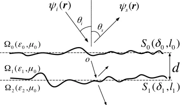
According to Fig. 1, the considered multilayer consists of two one-dimensional Gaussian rough interfaces. The upper one S0, separates a lossless homogeneous dielectric medium Ω0(ε0, µ0), with relative permittivity ε0 = 1 and permeability µ0 = 1, from a lossless medium Ω1(ε1, µ1 = µ0). This homogeneous medium fills a layer separated from the semi-infinite lower medium Ω2(ε2, µ2=µ0) by another rough
i θ ( )r
i
ψ
0(ε µ0, 0) Ω
1( ,ε µ1 0) Ω
( )
s
ψ r
2(ε µ2, 0) Ω
0( , )0 0
S
δ
l1( 1, )1 S δ l s
θ
d
o
surfaceS1. Each boundary is invariant with respect to any translation along the y axis. The height profiles of S0 and S1 are given by
z0 =f0(x) andz1 =f1(x) respectively. dis the average height between the two Gaussian rough interfaces.
For the case of a two media problem where the lower medium (Ω1) has permittivity ε1, the dual integral equation is needed. Let ψ0(r),
ψ1(r) be the field in Ω0 and Ω1, respectively. The fields in Ω0 and Ω1 satisfy the following equations:
ψi(r) =
1
2ψ0(r)−
P.V dsψ0
rnˆ·∇G0
r,r+
s dsG0
r,rnˆ·ψ0
r
(1)
1
2ψ1(r)+
P.V dsψ1
rnˆ·∇G1
r,r−
s dsG1
r,rnˆ· ∇ψ1
r= 0
(2)
Note thatG0(r,r) andG1(r,r) are the Green’s functions for Ω0 and Ω1, respectively.
G0
r,r=i 4H
(1) 0
k0r−r, G1
r,r=i 4H
(1) 0
k1r−r (3) where r is on the rough surface. The field ψ0(r), ψ1(r) satisfies the following equation based on boundary condition:
ψ0(r) = ψ1(r)|r∈S0 (4)
ˆ
n· ∇ψ0(r) =
ε0
ε1 ˆ
n· ∇ψ1(r)|r∈S0 (5)
where the normal vector on the rough surface ˆn = −√f 1+f2xˆ +
1 √
1+f2zˆ. The rough surface is discretized along thex axis and MOM
with point-matching is used. We can obtain the matrix equation from (1)–(2) as follows [16]:
A B C ρD ·
V1(x)
V2(x)
=
ψi(x)
0
(6)
where V1(x) = ψ0(r)|r∈S0, V2(x) = u(x) =
1 + (df0
dx)2( ˆn ·
of the matrix are shown below [17]:
Amn =
∆xκ(xm, xn) m=n i∆x
4
1 +i2
π ln
γk0 4e ∆lm
m=n (7a)
Bmn =
−∆xκN(xm, xn) m=n
1 2−
f0(xm)
4π
∆x
1 + (f0(xm))2
m=n (7b)
Cmn =
∆xκ1(xm, xn) m=n i∆x
4
1 +i2
π ln
γk1 4e ∆lm
m=n (7c)
Dmn =
−∆xκ1N(xm, xn) m=n
−1 2 −
f0(xm)
4π
∆x
1 + (f0(xm))2
m=n (7d)
where ∆lm = ∆x
1 + (f0(xm))2, γ = 1.78107, e = 2.71828138
and the wave number of Ω0 and Ω1 are k0 = ω√µ0ε0, k1 =
ω√µ1ε1, respectively. f0(x) and f0(x) are the first- and second-order differential of rough surface height function, respectively, and the detail expressions of κ, κN, κ1, κ1N are given in [15]. After solving the
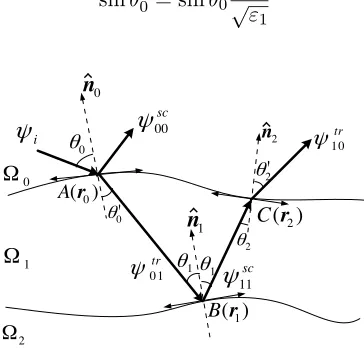
matrix Eq. (5), we can obtained the ψ0(r) and ˆn· ∇ψ0(r) without considering the transmitted field from Ω1. In order to calculate the total field ψ(r) of every point on the upper rough surface S0 with considering the transmitted field ψ10tr(r), it is necessary to derive the value of the transmitted fieldsψtr10(r) of every point. In the following, the Kirchhoff approximation is applied to derive the transmitted fields. The transmitted fieldsψtr10(r2) into Ω0 at the points C(r2) due to the rough upper and lower interfaces is calculated, as represented in Fig. 2. We consider that the upper and lower rough surfaces have on every point a large radius of curvature relative to the wavelength of the incident fields, λ0 and n1λ0, respectively, n1 being the index of refraction in Ω1. Under the condition, the tangent plane hypothesis is valid and Fresnel laws can be locally applied. Thus, at the pointA(r0) on S0, we consider the transmitted light ψ01tr. The transmitted field
ψtr01into Ω1 due to the incident field ψi(r0) is by
ψtr01(r0) = T01(r0)ψi(r0) (8a) ˆ
n0· ∇ψtr01(r0) = T01(r0)
∂ψi(r0) ∂n0
(8b)
where Tij = ρij(1 +Rij) is the Fresnel transmission coefficient. For
εi/εj
Rij
r=
cosθk−(εj/εi−sin2θk)1/2
cosθk+ (εj/εi−sin2θk)1/2
for horizontal polarization
εj/εicosθk−(εj/εi−sin2θk)1/2 εj/εicosθk+(εj/εi−sin2θk)1/2
for vertical polarization
(9)
and εi(j) is the relative permittivity of the medium Ωi(j) and θk=0,1,2 represents the local incidence angle as it is shown in Fig. 2. The transmitted beam fromA(r0) will intercept the lower interface at point
B(r1). It can be easily located with the Fresnel law: sinθ0= sinθ0
1 √ε 1 (10) 0 θ i
ψ
0 Ω 1 Ω 00 scψ
2 Ω 0 θ' 0 ( ) A r 1 ( ) B r 2 ( ) C r 0 n 10 tr ψ 0 1 tr ψ 11 scψ
1θ θ2
2 θ' 1 θ 2 n 1 n
Figure 2. Kirchhoff approximation.
Finally, the transmitted fieldψ10tr(r2) atC are [12]
ψ10tr(r2) =T10(r2)R12(r1)T01(r0)ψi(r0)e−
jk√ε1r2−r1+r1−r0
(11a)
ˆ
n2· ∇ψtr10(r2) = T10(r2)(−R12(r1))
T01(r0)
∂ψi(r0)
∂n0
e−jk
√ε
1r2−r1+r1−r0
(11b)
to determine numerically the locations of the pointsB andC for each point A(r0). It is easy for us to obtain the numerical pointBnum and Cnum using some simple method. Finally, ∆ϕis estimated by [12]
∆ϕ=k√ε1(ABnum+BnumCnum) (12)
Then we can get ψtr
10(r) and ˆn · ∇ψ10tr(r) for each point from Eq. (11). After obtaining ψ0(r) and ˆn· ∇ψ0(r) with MOM. Finally, the valuesψ0(r) andψ10tr(r) (if it exists) are added at each point ofS0, the total fields of each point ofS0 is
ψ(r) =ψ0(r) +ψtr10(r)|if exist (13) Notice that we calculate the Eq. (13) is to trace the ray reflected from the lower surface which means that in some regions of the upper surface there may be high density of such rays and other regions will have low density. This may be mainly due to the fact that in this paper, we are interested in the one-order Kirchhoff approximation where the multiple scattering phenomenon is neglected and to reduce the complexity of the hybrid method, the subsequent interactions between the two surfaces are ignored. Furthermore, these factors may introduce an error in the calculations especially for the calculation of the very rough layers. For the scattering computation, the two-layer surface realizations are needed at a set ofPpoints with spacing ∆xover length
L= P∆x. Realizations with the desired properties can be generated at pointsxp =p∆x(p= 1, . . . , P) using [14]
f0,1(xp) =
1
L
P 2−1
i=−P2
F(Ki) exp(jKixp) (14)
wheref0,1(xp) represents the height profiles of S0 andS1, respectively. Fori≥0,
F(Ki) =
2πLW(Ki)
[N(0,1) +jN(0,1)]/√2 i= 0, P/2
N(0,1) i= 0, P/2 (15)
and, for i <0, F(Ki) =F(K−i)∗. Ki = 2πi/Land each time N(0,1)
appears, which indicates an independent sample taken from a zero mean, unit variance Gaussian distribution. For the present work, the rough surface model used in scattering model is generated randomly with a Gaussian roughness spectrum, i.e., [14]
W(Ki) =
l0,1δ02,1/2 √
whereδ0,1 represents the rms height of the upper and lower surface (S0 and S1), respectively as well as the correlation lengthl0,1. Eq. (14) is computed with a fast Fourier transform (FFT). We can choose different values of the parameters (δ0,1 and l0,1) for upper and lower Gaussian
rough surface.
It should be noted that, in numerical simulation of scattering from rough surface, the tapered wave described by the tapering parameterg
has been employed to guard against the edge effects associated with the illuminated finite surface L. The tapered incident wave illuminating the composite model is given by [17]
ψi(r) = exp (−jk0(xsinθi−zcosθi) (1 +w(r)))
exp
−
x+ztanθi g
2
(17)
where g is the tapering parameter, θi is the incident angle. The
additional factor in the phase,w(r) is inserted such thatψi(r) obeys
the wave equation to a higher order. The choice ofw(r) is expressed as
w(r) =
2
x+ytanθi g
2 −1
(kgcosθi)2
(18)
Then we can write the analytical expression of the scattered field due to the rough upper and lower interfaces using Huygens’s principle (ψ(r0) represents the total field onS0)
ψs(r) =
S0
[ψ(r0) ˆn· ∇G0(r,r0)−G0(r,r0) ˆn·ψ(r0)]ds0 (19) The bistatic RCS σ(θs) in the direction ks is then calculated on the
far field as in [17]:
σ(θs) =
ψ(sN)
2
8πkgπ/2 cosθi
1− 1 + 2 tan 2θ
i
2k2g2cos2θ
i
(20)
with
ψ(sN)=
∞
−∞dx
ˆ
n·∇ψz=f0(x)
1+f0(x)2−ψ(x)ikf
0(x)sinθs−cosθs
3. NUMERICAL RESULTS AND DISCUSSIONS
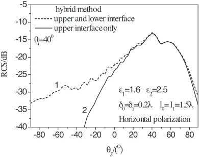
In all the following numerical implementations, both the relevant parameters of the Gaussian rough surface are measured in incident wavelength λ and the rough surface is created by 100 Monte Carlo realizations in the following numerical simulations. The average height between the two interfaces isd= 5λfor the scattering plots in Fig. 3–6. In the Fig. 3(a), We first illustrate the rough surface scattering from a two-layered Gaussian rough interfaces with the same parameters by the hybrid method and KA. The bistatic scattering coefficient of this two-layered Gaussian rough surface are computed by using the classical KA and the hybrid method, respectively. It is found that the scattering pattern by the hybrid method is in good agreement with that by KA near the specular angular range and there is great difference in the larger scattering angles. This indicates that the hybrid method is more exact than KA. We next illustrate in Fig. 3(b) rough surface scattering from a single- and two-layered system with Gaussian rough interfaces with the same parameters. It is easy for us to find that the bistatic scattering coefficient from two-layered system is larger than that from the single-layered system on the most scattering angles except for the specular direction. For the plot 1 in Fig. 3(b), the computing time of the numerical simulations is 65 s. Here, the rough surface is created by 1 Monte Carlo realization and the dominant frequency of CPU is 1.4 GHz.
To further explore the important scattering characteristic of the two-layer Gaussian rough surface model, the dependency of the bistatic scattering coefficient on relative permittivityε2is plotted for horizontal polarization by the hybrid algorithm in Fig. 4. The incident angles are θi = 20◦. The height rms of the upper and lower rough surface
are 0.1λ and the correlative length 1.2λ, respectively. It is observed that the bistatic scattering cross section of layered model increases with increasing ε2. It should be pointed out that as for the case of ε2 = ε1, the two-layer media can be regarded as the single-layer media, and the total scattered field in Ω0 only corresponds to the scattered field ψsc00(r0) in S0 due to the incident field. As for the case of ε2 = ε1 is concerned, the total scattered fields in Ω0 consists of
ψsc00(r0) in S0 and ψtr10(r) due to S1, which results that the bistatic scattering coefficient of layered model increases with the larger value of the relative permittivity ε2 in the lower media.
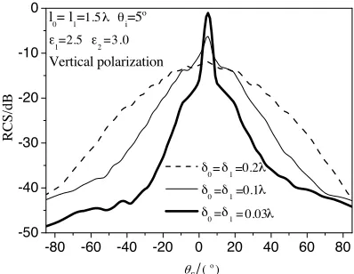
In Fig. 5, the effect of the height rms on the bistatic scattering coefficient of the two-layer Gaussian rough surface with the same parameters (δ0 = δ1, l0 = l1) is examined. The incident angles are
-80 -60 -40 -20 0 20 40 60 80 -30
-25 -20 -15 -10
θi=10 0
ε1=2.5 ε2=3.0
δ0=0.5λ δ1= 0.05λ l0= l1=1.5λ
Horizontal polarization hybrid method
KA
RC
S/
dB
S/(
Ο)
Figure 3a. Comparison of the hybrid method and KA for the two-layer model.
-80 -60 -40 -20 0 20 40 60 80 -40
-35 -30 -25 -20 -15 -10 -5
θi=40 0
ε1=1.6 ε2=2.5
δ0=δ1=0.2λ l0= l1=1.5λ Horizontal polarization hybrid method
upper and lower interface upper interface only
RC
S/
dB
S/(
Ο) 1
2
Figure 3b. The bistatic scattering coefficient of the single and two-layer model.
respectively. The correlative length is 1.5λ. It is observed that the bistatic scattering coefficient increases with increasingδover the most angular range except for the specular direction. It is mainly due to the fact that the two-layer rough surface can be regarded as two flat interfaces for the small value height rms, which results in the obvious peaks on the specular direction (corresponding to the strong coherent scattering) and weak incoherent scattering in the angular range far from the specular direction.
-80 -60 -40 -20 0 20 40 60 80 -60
-50 -40 -30 -20 -10
ε2=50
ε2=20
ε2=2.0
ε2=1.6
ε1=1.6 θi=20o δ0 δ1=0.1λ l0= l1=1.2λ
Horizontal polarization
RCS/dB
θS (o)
/
=
Figure 4. The bistatic scattering coefficient of the two-layer model versusε2.
-80 -60 -40 -20 0 20 40 60 80 -50
-40 -30 -20 -10 0
l
0= l1=1.5λ θi=5 o
ε1=2.5 ε2=3.0 Vertical polarization
δ0 δ1 λ δ0 δ1 λ δ0 δ1
RC
S/
d
B
=
=
= =
=
= 0.2
0.1
λ
0.03
θS (
o)
/
Figure 5. The bistatic scattering coefficient of the two-layer model versusδ.
scattering coefficient of the two-layer Gaussian rough surface with the same parameters (δ0 = δ1, l0 = l1) for horizontal polarization is depicted. The incident angles areθi = 10◦. The relative permittivity
of Ω1 and Ω2 are as same as ones in Fig. 5. The rms height ofS0 and
-80 -60 -40 -20 0 20 40 60 80 -40
-30 -20 -10
l
0= l1= 1.0λ l
0= l1=1.5λ l0= l1= 2.0λ δ0=δ1=0.2λ θi=10
o
ε1=2.5ε2=3.0 Horizontal polarization
RCS/dB
θS (
o
)
/
Figure 6. The bistatic scattering coefficient of the two-layer model versusl.
-80 -60 -40 -20 0 20 40 60 80 -40
-35 -30 -25 -20 -15 -10
d=2 0λ d=1 0λ d=5λ
δ0=δ1 l0= l1=1.5λ
θi=10o
ε1 ε2
Harizontal polarization
RCS/dB
=0.2λ
=2.5 =3.0
θS (
o
)
/
Figure 7. The bistatic scattering coefficient of the two-layer model versusd.
scattered energy. This implies a decrease of the scattered energy in the specular direction and a increase of the incoherent scattering (the heavy line shown as in Fig. 6). The rough surface scattering from two-layered system with the different heightsdbetween the two interfaces for horizontal polarization are also present in Fig. 7. The height rms of the upper and lower rough surface are both 0.3λand the correlative length 1.5λ, respectively. The incident angle isθi = 10◦and the relative
that the bistatic scattering coefficient is not sensitive to the varying of the average height between the two interface.
4. CONCLUSION
To investigate the bistatic scattering from a stake of two one-dimensional Gaussian rough surface, a hybrid algorithm combining the method of moments with the Kirchhoff Approximation is developed. This approach presents overcomes the problem of inaccuracy when using the first-order Kirchhoff Approximation in some degree due to the fact that the scattered fields from the upper rough sea surface is solved by the MOM. The advantage of this hybrid method is performed in the numerical results compared with that by KA. Finally, the influence of the relative permittivity, the height rms and the correlative length, the average heights between the two interfaces on the bistatic scattering coefficient is discussed in detail. It is remained for us to calculate the scattering from two-layer lossy dielectric rough surface using this hybrid method which has more significance.
REFERENCES
1. Wismann, V., M. Gade, W. Alpers, and H. H¨uhnerfuss, “Radar signatures of marine mineral oil spills measured by an airborne multi-radar,” Int. J. Remote Sens., Vol. 19, No. 3, 3607–3623, 2005.
2. Blumberg, D. G., et al., “Soil moisture assessment by an airborne scatterometer in Chernobyl disaster area and Negev Desert,”
IGARSS 2000, IEEE 2000 International, Vol. 5, 2011–2013, 2000. 3. Chen, K.-S., A. K. Fung, J. C. Shi, and H.-W. Lee, “Intepretation of backscattering mechanisms from non-Gaussian correlated randomly rough surfaces,” J. of Electromagn. Waves and Appl., Vol. 20, No. 1, 105–118, 2006.
4. Fung, A. K. and N. C. Kuo, “Backscattering from multi-scale and exponentially correlated surfaces,”J. of Electromagn. Waves and Appl., Vol. 20, No. 1, 3–11, 2006.
5. Sanchez-Gil, J. A., A. A. Maradudin, J. Q. Lu, and V. D. Freilikher, “New features in the transmission of light through thin metal films with randomly rough surfaces,” Geoscience and Remote Sensing Symposium, Vol. 1, 273–276, 1994.
6. Ho, M., “Scattering of electromagnetic waves from vibrating per-fect surfaces: simulation using relativistic boundary conditions,”
7. Pinel, N. and C. Bourlier, “Modeling of the bistatic electromag-netic scattering from sea surfaces covered in oil for microwave ap-plications,”IEEE Transactions on Geoscience and Remote Sens-ing, Vol. 46, No. 2, 385–392, 2008.
8. Ren, Y.-C. and L.-X. Guo, “Study on the multiple scattering and shadowing effect from the two-dimensional rough surface,”
Systems Engineering and Electronics, Vol. 28, No. 4, 496–507, 2006.
9. Guo, L.-X. and Z.-S. Wu, “Fractal characteristics investigation of electromagnetic scattering from 2D conducting rough surface,”
Acta Physica Sinica, Vol. 49, No. 6, 1065–1069, 2000.
10. Fuks, I. M. and A. Voronovitch, “Wave diffraction by rough interfaces in an arbitrary plane-layered medium,” Waves in Random Media, Vol. 10, S253–S272, 2000.
11. Pinel, N. and C. Bourlier, ‘ “Scattering from very rough layers under the geometric optics approximation: Further investigation,”
Journal of the Optical Society of America A, Vol. 25, No. 6, 1293– 1306, 2008.
12. D´echamps, N. C., et al., “Numerical simulations of scattering from one-dimensional rough intefaces,” Proceedings. 2003 IEEE International, Vol. 1, 118–120, 2003.
13. Ogilvy, J. A., Theory of Wave Scattering from Random Rough Surface,IOP Publishing, Bristol, 1991.
14. Thorsos, E., “The validity of the Kirchhoff approximation for rough surface scattering using a Gaussian roughness spectrum,”
J. Acoust. Soc. Am., Vol. 83, 78–91, 1988.
15. Beckman, P. and A. Spizzichino, The Scattering of Electromag-netic Waves from Rough Surface, Pergamon, London, 1963. 16. Wang, X., C.-F. Wang, and Y.-B. Gan, “Electromagnetic
scattering from a circular target above or below rough surface,”
Progress In Electromagnetics Research, PIER 40, 207–227, 2003. 17. Tsang, L., J. A. Kong, and K. H. Ding, Scattering of