Analyzing algorithm precision for Stock Market datasets

(1)

Available online: https://edupediapublications.org/journals/index.php/IJR/ P a g e | 692

Analyzing algorithm precision for Stock Market datasets

K. Brah

_m

a Naidu,

Surapaneni Divya Sri , Domakonda Abhigna , Aitipamula Harika

1

_{Assistant Professor, Department of Computer Science and Engineering)}

BVRIT Hyderabad College of Engineering for Women

2_{Department of Computer Science BVRIT Hyderabad Hyderabad, India}

[email protected] , [email protected] , [email protected]

Abstract- The analysis proposed in this paper is a result of observation from our extensive and rigorous study, for analyzing the algorithmic precision of supervised machine learning algorithms. The usage of machine learning algorithms is done in order to find the predictive capabilities for a handful models for time series analysis using stock market datasets. This is done by the usage of scientific tools available in Python such as Web API’s for Data retrieval, Pandas, Training and Testing methods. Here, stock market datasets are used for checking the accuracy of predictive precision by means of numerical data. The main aim is to identify which algorithm best suits for numeric analysis, in terms of accuracy and less erroneous results while prediction.

Keywords- Algorithms, analysis, prediction, stock market, datasets, numerical data, scientific computing, Python, time series, machine learning, supervised learning

INTRODUCTION

Prediction of future events is a very interesting aspect. This is mainly useful when there’s a need to carefully invest. Bad investments lead to a huge loss and can take a toll on the econometric cycle. The focal reason is to learn machine learning algorithm efficiencies. The need for financial analysis for profit is most sought after these days. The guidance to right investment can lead to mutual profits [4].

Since, there are several algorithms it is hard to decide upon just one for practical real-time usage. In order to forgo the difficulty while choosing from a vast range of algorithms, an analysis of 5 algorithms is done. The use of ARIMA, Linear Regression, Logistic Regression, LSTM (Long-short term memory) and k-Nearest Neighbors (kNN) is done here. The key aspect is to settle upon an algorithm that provides highest precision and accuracy while prediction. Time series analysis

of data for a certain period of time can be done to achieve desired results.

MACHINE LEARNING ALGORITHMS

The Machine Learning is a kind of application that provides a system a certain set of capabilities and experiences to learn from. It consists of artificial intelligence (AI) that provides systems the ability to automatically learn and improve from experience without being explicitly programmed. It focuses on the development of computer programs that can access data and use it to learn for themselves. The primary aim is to let the computer learn automatically without human intervention, assistance and training. Also, this helps it to learn to act accordingly as per need.

The classification of Machine Learning algorithms is done as:

Supervised Learning – most popular approach that makes predictions based on a set of examples. Here the system is trained first and then tested

Unsupervised Learning – data points have no labels associated with them. Instead, the goal is to organize the data in some way or to describe its structure. This can mean grouping it into clusters or finding different ways of looking at complex data so that it appears simpler or more organized. Here, the system is not trained but only tested

Semi Supervised Learning – the system needs both the supervised and unsupervised methods while learning, and

(2)

ALGORITHMS

There are various algorithms in Machine Learning which have a varied usage scope. Linear regression, Logistic regression, k-Nearest Neighbours, Apriori, Decision Tree, Random Forest, Gradient Boost, Support Vector Machine, Naïve Bayes, K-Means, Dimensionality Reduction, Markov Decision process, etc are some of the algorithms available for various aspects of Machine Learning purposes. The proper usage of the right algorithm can yield desired results. The choice of the algorithm to be used is based on several factors like what we want to achieve, what shall be the data set provided to the system, what are the attributes that determine our outcome from the system, the most significant attributes in the data set and what do we expect it to do.

The considerations that need to be made while choosing a machine learning algorithm are listed as follows:

Accuracy

Getting the most accurate answer possible isn't always necessary. Sometimes an approximation is adequate, depending on what you want to use it for. If that's the case, you may be able to cut your processing time dramatically by sticking with more approximate methods. Another advantage of more approximate methods is that they naturally tend to avoid over-fitting.

Training time

The number of minutes or hours necessary to train a model varies a great deal between algorithms. Training time is often closely tied to accuracy—one typically accompanies the other. In addition, some algorithms are more sensitive to the number of data points than others. When time is limited it can drive the choice of algorithm, especially when the data set is large.

Linearity

Lots of machine learning algorithms make use of linearity. Linear classification algorithms assume that classes can be separated by a straight line (or its higher-dimensional analog). These include logistic regression and support vector machines (as implemented in Azure Machine Learning). Linear regression algorithms assume that data trends follow a straight line. These assumptions aren't bad for some problems, but on others they bring accuracy down

Number of parameters

Parameters are the knobs a data scientist gets to turn when setting up an algorithm. They are numbers that affect the algorithm's behavior, such as error tolerance or number of iterations, or options between variants of how the algorithm behaves. The training time and accuracy of the algorithm can sometimes be quite sensitive to getting just the right settings. Typically, algorithms with large numbers parameters require the most trial and error to find a good combination.

Number of features

For certain types of data, the number of features can be very large compared to the number of data points. This is often the case with genetics or textual data. The large number of features can bog down some learning algorithms, making training time unfeasibly long.

Once these factors are properly sorted and decided upon, it becomes easy to zero in upon choosing the perfect algorithm. [2]

IMPLEMENTATION

The implementation of all the five tried models is given below. The accuracy of prediction is tested against Microsoft datasets for the period (1986-03-13 to 2018-03-12) i.e, March 13th_{1986 to March 12}th_{2018. The results of each is noted}

and analysis is made as to which is the best algorithm to choose based on the accuracy.

ARIMA Model

The ARIMA (Auto Regression Integrated Moving Averages) Model is a model that better understands time series data and predicts points in the future. Its main application is in the area of short term forecasting requiring at least 40 historical data points. The ARIMA model is depicted as

ARIMA(p,d,q) …(1)

p – depicts simple regression with an indeprendant variable

d – represents number of differentiations of time series, to make them stationary

(3)

In order to test the data to find auto-correlation in the time series, Durbin Watson Test is performed. The presence of positive auto-correlation is depicted between (0<2) and a negative auto-correlation between (2<4) [1].

For the analysis of this model, we have used the Microsoft data which has been obtained using the Yahoo Web API. Now a data space for a certain time period is declared and is retrieved using Pandas. Since the data is usually raw and may contain gaps and unevenness, ‘ffill method’ is used to even out the missing data. The previous days data is added in place of the empty record places. Also, the least significant columns are removed, mainly retaining the Close Price of the Stock. This is done to reduce errors.

The data is then spilt for training and testing(some used for prediction purposes). Also, the lags between the values in the time series are checked through auto correlation and partial auto correlation. This accounts to the stationary feature in the time series which makes it eligible for use in the ARIMA model. In place of the above test, Ad-fuller test can be performed to check the stationarity of the time series.

In our approach, we have used ARIMA(1,1,1) as we do not want the attribute of a specific data point to affect the attributes if another data point in the future. This gives rise to the predicted values lying well inside the confidence interval with minute errors. Also, Naïve Benchmark is used by shifting the original data by 1. This gives the last days forecast for next day.

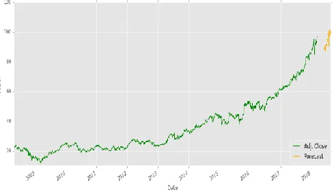
The observed accuracy for this model is 98.77% in accordance to Microsoft data sets.

Figure 1: Actual close price vs Forecasted price for MSFT dataset using ARIMA

Linear Regression

Linear regression is a basic and commonly used type of predictive analysis. The overall idea of regression is to examine two things: (1) does a set of predictor variables do a good job in predicting an outcome (dependent) variable? (2) Which variables in particular are significant predictors of the outcome variable, and in what way do they–indicated by the magnitude and sign of the beta estimates–impact the outcome variable? These regression estimates are used to explain the relationship between one dependent variable and one or more independent variables [3].

The simplest form of the regression equation with one dependent and one independent variable is defined by the formula

y = c + b*x …(2)

y = estimated dependent variable score,

c = constant,

b = regression coefficient, and

x = score on the independent variable.

Three major uses for regression analysis are (1) determining the strength of predictors, (2) forecasting an effect, and (3) trend forecasting. [2]

For the analysis of this model, we use Pandas, Numpy and Quandl to load a data frame. To get a peek into the data, we use the head function where we view each row and column attributes.

Now, feature engineering is done to extract the most relatively likely features that shall be used for the analysis. Now, we chose a column for forecasting of the data and pick a certain number of days to be forecasted.

(4)

Python libraries. Then, the prediction for the next 30 days of data is done as a function of dates.

The actual graph is plotted and against this, the prediction is also plotted. It can be observed that the Linear Regression does a pretty good job while analyzing the accuracy but does not stay up to mark as when compared to the ARIMA model predictions. This may account to the non-stationary behavior of the data set in the time series. Since, we do not perform auto correlation on the data set in this approach, this model gives slightly less accurate results for the same data set. The observed accuracy for this model is 98.66% in accordance to Microsoft data sets.

Figure 2: Price prediction for MSFT dataset using Linear Regression

Logistic Regression

Logistic Regression is the appropriate regression analysis to conduct when the dependent variable is dichotomous (binary). Like all regression analyses, the logistic regression is a predictive analysis. It is used to describe data and to explain the relationship between one dependent binary variable and one or more nominal, ordinal, interval or ratio-level independent variables.

The sigmoid/logistic function is given by the following equation [5]

y = 1 / 1+ e-x _…(3)

In this approach, the data is imported using Yahoo finance by usage of pandas_data_reader. The Microsoft stock data is loaded for a certain time period and only the relevant column attributes are viewed.

We then define the predictor variables by using 10-day moving average, correlation, relative strength index, and the difference between consecutive days’ price. Then, the Target variable is defined.

Further, the data frame is split in a 70:30 ratio, where 70% is used for training and 30% is used for testing purposes. We will instantiate the logistic regression using ‘LogisticRegression’ function and fit the model on the

training dataset using ‘fit’ function. Then, the coefficients are examined.

The model is now evaluated by the usage of Confusion Matrix where the true values for the data set are known. We then check for the model accuracy. On a final note, a 10-fold cross validation is done to check for the correctness of the given accuracy. Then the original returns and the strategy returns are plotted against one another to check for efficiency of result.

The observed accuracy for this model is around 50.84% in accordance to Microsoft data set.

Figure 3: Returns of Microsoft charted against the Strategic returns of Logistic regression.

K – Nearest Neighbor

KNN makes predictions using the training dataset directly.

(5)

To determine which of the K instances in the training dataset are most similar to a new input a distance measure is used. For real-valued input variables, the most popular distance measure is Euclidean Distance.

Euclidean distance is calculated as the square root of the sum of the squared differences between a new point (x) and an existing point (xi) across all input attributes j [6]

Euclidean Distance(x, xi) = sqrt( sum( (xj – xij)^2 ) ) …(4)

KNN can be used for both classification and regression predictive problems. However, it is more widely used in classification problems in the industry. The kNN algorithm is an extreme form of instance-based methods because all training observations are retained as part of the model.

The analyze this algorithm, we first load the data in a csv file format and then randomly split it into train/test sets, the standard ratio being 67:33.

In order to make predictions we need to calculate the similarity between any two given data instances. This is needed so that we can locate the k most similar data instances in the training dataset for a given member of the test dataset and in turn make a prediction. Through this, the Euclidean distance function is defined. Now that we have a similarity measure, we can use it collect the k most similar instances for a given unseen instance. This is a straight forward process of calculating the distance for all instances and selecting a subset with the smallest distance values [7].

Once we have located the most similar neighbors for a test instance, the next task is to devise a predicted response based on those neighbors. We can do this by allowing each neighbor to vote for their class attribute, and take the majority vote as the prediction. This voting is done by introducing a process function with some test neighbors.

An easy way to evaluate the accuracy of the model is to calculate a ratio of the total correct predictions out of all predictions made, called the classification accuracy. A function, getAccuracy sums the total correct predictions and returns the accuracy as a percentage of correct classifications. This function can be tested with dataset and predictions. The generated predictions are compared to the actual value in the test set.

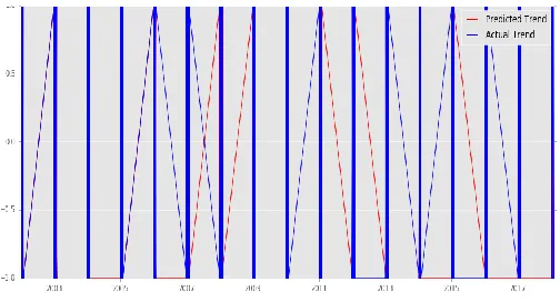
The observed accuracy of this model is about 66.06% in accordance to the Microsoft data set.

Figure 4: Prediction vs Actual Trend for MSFT data set using KNN

LSTM (Long Short Term Memory)

This model refers to a short term memory that can last for a long period of time. It is well-suited to classify, process and predict time series given time lags for unknownsize and duration between important events.

A common LSTM unit is composed of a cell, an input gate, an output gate and a forget gate. The cell is responsible for "remembering" values over arbitrary time intervals; hence the word "memory" in LSTM. Each of the three gates can be thought of as a "conventional" artificial neuron, as in a multi-layer (or feedforward) neural network: that is, they compute an activation (using an activation function) of a weighted sum. [14]

In order to analyze this algorithm, we perform the operations in the way of specification. First, we import all the required libraries and convert an array of values into a matrix format. Then, a seed for reproducibility is fixed and the dataset is normalized after being loaded.

(6)

The observed accuracy for this model is around 99.36% for the MSFT data set.

Figure 5: Baseline vs Efficiency for MSFT data set using LSTM

CODE

The code for the above results and procedure has been pushed into Google Drive and the link is shared below for reference. In order to clearly view and run the files, a version of Python 2.7 and JuPyter Notebook are required before running each python file.

https://drive.google.com/open?id=0B792_mC 8FN8bNTZjY0NxREl2c0VQZUQ5OUFnTVFVS3BidE5z

CONCLUSION

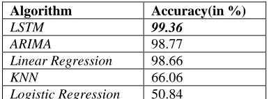
Algorithm Accuracy(in %)

LSTM 99.36

ARIMA 98.77

Linear Regression 98.66

KNN 66.06

Logistic Regression 50.84

Table 1: Accuracy of each algorithm for MSFT Dataset

Through the tabulated results, it is clearly evident that the LSTM model best suits for the chosen, Microsoft data set. The highest accuracy is achieved through this model, followed by the ARIMA model. Below is a point-wise analysis of what is analyzed to be the cause of the given percentages of accuracy.

 The highest prediction accuracy is achieved by LSTM which is a recurrent neural network that is trained using Backpropagation through time and

vanishing gradient problem. It’s use falls in creating large recurrent networks that can be used to address difficult sequence problems to achieve state-of-the-art results. The netwroks of LSTM consist of units which are like mini state machines where the gates of the units have weights that are learned during the training process. Hence, the precision is basically very high.

 The high precision of prediction for the ARIMA model can be attributed to the stationarity that is achieved in the data set before analysis and prediction are done. This smoothens out noise, redundancies, null values and missing data from the chosen data set. For, the Microsoft data set chosen here, ARIMA(1,1,1) is the best analysis model, since the attributes of a specific data point do not affect the other data points any time in the future.

 In case of Linear regression, the success is attributed to its feature extraction process, which eliminates all possible redundancies. The feature which is the most relevant and suitably required for analysis is extracted or considered. All the other features are discarded. The extracted feature represents the most significant attribute that can chart the perfect prediction in terms of accuracy.

 The k-Nearest Neighbors algorithm has a considerable accuracy, but it lacks higher efficiency because the algorithms approach may not suit the dataset. The algorithm tends to choose similar data from the dataset and measure the distance from a predefined variable. The data chosen may not have many similarities or maybe no similarities at all. The analysis of the Microsoft dataset makes it clear since there’s not much of closeness or evenness observed in it.

 Logistic regression holds lowest accuracy of prediction among all the chosen algorithms. This is attributed to the nature of its execution. In this method, since there’s one dependent variable and one or more independent variable it is spurious to zero in on one of the most probable variables. Also, some factors may affect one another and attributes of the dependent and independent variables may not be in acceptance of one another.

(7)

REFERENCES

[1] Ping Feng Pai, Chih Sheng Lin, September 2004, Da-Yeh University, Taiwan, “A Hybrid ARIMA and support vector machines model in stock price forecasting”

[2] George S. Atsalakisa_,_{Kimon P. Valavanis}b_{, a Technical}

University of Crete, Greece, b University of South Florida, USA, July 2008, “Surveying Stock market forecasting techniques-Part II Soft Computing methods”

[3] Richard A. Johnson, Dean Wichern, September 2015,

Multivariate Analysis

[4] Joel Hasbrouck, May 2015, “The Review of Financial Studies”, Volume 4, Issue 3, 1 July 1991, Pages 571–595, “The Summary Informativeness of Stock Trade: An Econometric Analysis”

[5] David W. Hosmer, Stanley Lemesbow, June 2007,

Goodness of fit tests for the multiple logistic regression model.

[6] Khalid Alkhatib, Hassan Najadat, Ismail Hmeidi, Mohammed K. Ali Shatnawi, Mar 2013, Jordan University of Science and Technology, Jordan, Stock Price Prediction using k-Nearest neighbor(kNN) algorithm

[7] Sadegh Bafandeh Imandoust, Mohammad Bolandraftar,

Oct 2013, Payame Noor University, Iran, “Application of k-Nearest Neighbor(kNN) approach for predicting economic events: Theoritical Background”

[8] analyticsvidhya.com

[9] machinelearningmastery.com

[10] suruchifialoke.com

[11] quantinsti.com

[12] agounaris.eu

[13] github.com/sammanthp007

[14]https://en.wikipedia.org/wiki/Long_sh ort-term_memory

[15]https://machinelearningmastery.com/tim