System Failure Prediction using Log Analysis

38 | P a g e

System Failure Prediction using Log Analysis

1

Animesh Dutta

Anurag Sharma

1

Department of Information Technology, Kalyani Government Engineering College (India)

2

Data Scientist, Celebal Technologies

ABSTRACT

In modern days, system failure is a grave issue and needs to be dealt with. IT companies or various research organizations can be highly benefited if an accurate system failure prediction can be obtained. The adverse effect of computer failure is somewhat mitigated if a proper prediction is made beforehand. The usage of resources, applications and other memory consuming processes can be limited if such a case is about to occur thus preventing the system breakdown.

Achieving accurate predictions with adequate time left is quite difficult. In this paper, we present a simple approach to detect the failure by parsing the log files quite in advance. We generate an early warning before a failure condition arises. To serve our purpose, we have used a Recurrent Neural Network, namely, Long Short-Term Memory. The approach in this paper uses a sliding window to fetch the desired results. The important factors taken into account being RAM, CPU and Hard Disk utilization.

Keywords - Deep Learning, Log Analysis, LSTM, Recurrent Neural Network, System Failure Prediction

1. INTRODUCTION

With recent emerging technologies in computing, we have seen tremendous dependence on these to serve a variety of

critical services. Sectors such as banking, research organizations and railway/flight reservation portals rely on computer

systems. It is quite clear that reducing the downtime of these systems is extremely important and can be vital for various

operations in day to day life. Various examples have portrayed the impact of disruption from a computing failure. For

instance, in March 2008, a computing failure in the baggage system at Heathrow airport is estimated to have cost $32

million and affected 140,000 people [1].

Console logs or the logs generated in .nmon format for Linux systems have a piece of descriptive information that we

have used here to serve our purpose.

System Failure Prediction is essential in many applications like where a computer needs to perform high computations.

39 | P a g e

efficiently. The recovery of HPC can take long or even might not be possible at times. As per the research conducted at

the University of Toronto, their data shows that by far the most common types of hardware failures for HPC are due to

problems with memory or CPU. 20% of hardware failures are attributed to memory and 40% are attributed to CPU.

Hence this approach can help us to fully utilize the potential of HPC and alert a user before system failure arises. There

have been several approaches to system failure prediction. Some of them include Bayes networks, Hidden Markov

Models (HMM), Partially Observable Markov Decision Process (POMDP), Support Vector Machines (SVMs). [2,3]

The use of time series forecasting has been common too but it didn‘t include the parameters that we are going to state

next which can be beneficial.

The rest of the paper is divided is structured as follows. Section 2 consists of a description of .nmon extension log files generated from a system and the process of extracting the CPU, RAM and Hard disk utilization from the various

parameters.

Log files obtained from systems comprises of information on the status and memory consumption of a system. We

know that three main utilizations of a computer are CPU, RAM, and hard disk utilization. These log files can provide us

with timestamps and the exact utilization of resources on definite timestamps. We have taken into account the values at

timestamps with the same interval.

We had a data comprising of the log files of a system generated in the past five days in .nmon format. The timestamp variation considered is fixed and has a fixed gap of 10 minutes.

2. PROPOSED METHODOLOGIES

2.1. System Log Files (Parameters reduction)

In computing, log files are the ones which keep track of all the events occurring in an operating system. Most operating

systems include a logging system. System log files enable a dedicated, system to generate, filter and analyze log

messages. These files are essential to study the consumption of various resources while processes are executed in a

computer system. System log files give the status of a particular process such as security problems or system errors. By

reviewing the log files, the user can figure out the reason for any issue arising or whether all required processes are

loading properly. It contains information about the software, hardware and system components.

40 | P a g e

Table 1: CPU utilization

User%: This states that the processor is spending x% of its time running user space processes. A

user-space process is one that doesn‘t use kernel. Some common user-user-space process includes shells,

compilers, databases and all programs related to desktop. If the processor isn‘t idle then usually

the majority of CPU time is used to run user space processes.

Sys%: This states that the processor is spending x% of its time running user space processes. A

user-space process is one that doesn‘t use kernel. Some common user-user-space process includes shells, compilers, databases and all programs related to desktop. If the processor isn‘t idle then usually the majority of CPU time is used to run user space processes.

Wait%: This states that the processor is spending x% of its time running kernel processes. All the

processes and system resources are handled by the Linux kernel. The kernel performs tasks like

running system processes managing hardware devices like a hard disk in kernel space.

Idle%: This shows what percentage of CPU is waiting for other processes to complete. At times, the

processor might initiate a read/write operation and needs to wait for other processes to finish.

Hence we can see in Table 1, Idle% doesn‘t contribute to CPU utilization. Adding User%, Sys% and Wait% gives us the percentage of CPU utilization at that particular timestamp.

CPU utilization = User% + Sys% + Wait% (1)

We take the logarithmic value to keep the value small i.e between 0 and 2. For example,

log(1) = 0 (CPU is mainly idle) log(100) = 2 (CPU is fully utilized)

2.1.2. RAM utilization

Ram or Random Access Memory is a computer data storage used to store working data or machine code. Even though a

computer might have 16 GB or more RAM, excessive usage of memory has been causing an immense problem which

might lead to system crash.

High RAM usage can lead to many issues. The major causes for a high RAM usage being too many startup

41 | P a g e

Table 2: Memory nomenclature for RAM

MemTotal Total usable memory

MemFree The amount of physical memory not used by the system

Buffers Memory in buffer cache, so relatively temporary storage for raw disk blocks.

Cached Memory in the page cache (Diskcache and Shared Memory)

Table 2 shows common memory notations. We can calculate total memory used using the formula:

MemUsed = MemTotal-MemFree-Buffers-Cached (2)

% of used RAM at a particular timestamp = (MemUsed/MemTotal) * 100 (3)

2.1.3. Hard disk utilization

A hard disk or is an electromechanical data storage device to store and retrieve digital information. In Linux, we can get

the hard disk utilization by various drives using ‗df -h‘ command. This gives the percentage use of a particular drive.

Suppose a write operation is taking place in a hard disk and memory of Hard disk is constantly getting filled. We can

get the free space of hard disk at any timestamp. Subtracting this from the total hard disk memory provides the hard

disk space in use.

Hard disk utilization %= (Hard disk space used/ total hard disk space) *100 (4)

2.2. PCA

Now we have our values for CPU, RAM and hard disk utilization for timestamps. We apply PCA to get a single

reduced value out of these 3 parameters. As we know PCA or Principal Component Analysis is a way to deal with

highly correlated variables. We can get a single value for all the utilizations stated above. We can then apply univariate

time series forecasting to predict a single value for the future timestamps. We have applied the covariance matrix method to compute PCA.

The covariance matrix is a matrix whose element in j, k position is calculated as the covariance between jth and kth

elements of a random vector.

42 | P a g e

VΣ = λV

where V and λ in equation 5 represent the eigenvectors and eigenvalues of the covariance matrix, respectively.

The eigenvalues are scalar. [4] The eigenvectors are non-zero vectors representing the principal components (PCs), i.e.

each eigenvector represents one PC. The eigenvectors state the direction of PCA space while the eigenvalue represents

the length, magnitude or robustness of eigenvectors. The eigenvector which has the highest scalar value is used to

depict the first principal component and has maximum variance.

Steps for applying PCA:

a) Standardized the data.

b) Calculate the eigenvalues and eigenvectors from the covariance matrix. c) Sort the eigenvalues in decreasing order to rank corresponding eigenvectors.

d) Select 1 eigenvector corresponding to the largest eigenvalue. This gave us the reduced parameter for each timestamp.

2.3. Using LSTM to predict the value at future timestamps (univariate time series forecasting):

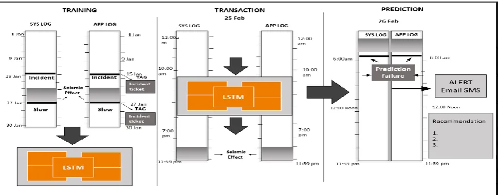
Fig. 1 briefly summarizes the approach we‘ve used in our paper. We‘ve let a moving window run on the log files and

fed it as inputs to the LSTM. On getting a high value of RAM, CPU and Hard disk utilization, a seismic effect is

generated and we can then send an Email or SMS alert to the user if we obtain a failure prediction.

Fig 1: Basic working principle of our model

LSTM or Long Short-Term Memory is an artificial Neural Network architecture used in the field of Deep Learning. A

43 | P a g e

controls the flow of input activations in the memory cell and the output gate controls output flow of cell activations.

An LSTM network computes a mapping from an input sequence x = (x1, ..., xT ) to an output sequence y = (y1, ..., yT )

by calculating the network unit activations using the following equations iteratively

From equations (6,7,8) i, f and o, are called input, forget and output gates respectively. W is the recurrent connection at

the previously hidden layer and current hidden layer, U is the weight matrix connecting the inputs to the current hidden

layer. σ is the sigmoid function which squashes the value of a function between 0 and 1.

From equation (9), is a ―candidate‖ hidden state that is computed based on the current input and the previous hidden

state. From equation (10), C is the internal memory unit, tanh being the activation function used.

We have denoted * as element-wise multiplication and ignored bias term, the hidden state ht as mentioned in equation

(11) is calculated by LSTM. [5]

The steps we followed:

i) A moving forward window of size 50, which means we used the first 50 data points as out input X to predict Y

i.e. 51st data point. Using the window from 1st _{to 51}st _{point next, we forecast for the 52}nd _point.

ii) A two-layered LSTM model combined with a dense output layer was used to make the prediction.

iii) We used the following two approaches to predict the output — 

a) We forecasted the value for each item in the test dataset.

b) We feed the forecast which was made previously back to the input window by moving it a step forward and make a

forecast at the timestamp needed.

We have a 3D input vector for the LSTM comprising of a number of samples, number of timestamps, number of

features.[6]

After saving the weights for the model trained, we plot the predicted values to visualize the trend in data. We have the

model with a 2 layered LSTM and a dense output layer at the end as shown in table 3 below. We use dropout in

44 | P a g e

Table 3:

LSTM Model summary :

Thus using this trained LSTM model, we obtained the results for various timestamps. The result wasn‘t exactly accurate

as we trained on a dataset consisting of log files for just 5 days. This can be more accurate if we have stored the log

files for a longer duration.

3. RESULTS

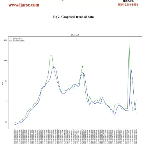
Fig 2 displays the graphical view of predicted values and actual values to find the trend. Despite the less amount of

training data, we got the desired variations in output. Our model was able to capture the trend. With more training data,

more accurate results can be predicted.

The green line represents the actual values while the blue line represents the predicted values. On X-axis, we have the

dates with a timestamp gap of 10 minutes. The Y-axis is the PCA reduced value which we earlier obtained.

The saved weights help us to predict the reduced values for future timestamps. Having the timestamps and PCA

reduced value for failure cases (can be noted for some cases where actual system failure took place), we can correctly

classify whether the predicted value falls in failure class or not. We used the Logistic regression classification algorithm

45 | P a g e

Fig 2: Graphical trend of data

4. CONCLUSION

This paper will help users to prevent system failure as it can send an alert mail or SMS to the person before the actual

failure takes place. The user can then limit the number of running processes on the system by terminating redundant

processes. Using LSTMs for time series forecasting helped us to get the reduced values for future timestamps. Then that

value was classified as Normal or Failure class using the Logistic Regression Classification model.

This work can be extended if we can add some more features to the existing list. We have just considered CPU, RAM

46 | P a g e

better accuracy.

5. ACKNOWLEDGMENT

This research was supported by Celebal Technologies. We thank our colleagues from Celebal Technologies who

provided insights and expertise that assisted the research. We would also take this opportunity to thank Mr. Anirudh

Kala, Co-Founder of Celebal Technologies for his assistance throughout and comments that greatly improved the

research paper.

6. REFERENCES

1. R. Charette and J. Romero, ―The staggering impact of it systems gone wrong,‖ IEEE Spectrum.

2. XUE, Z., DONG, X., MA, S., AND DONG, W. A survey on failure prediction of large-scale server clusters. In

Proceedings of the International Conference on Software Engineering, Artificial Intelligence, Networking, and

Parallel/Distributed Computing (2007), pp. 733–738.

3. Errin W. Fulp, Glenn A. Fink, and Jereme N. Haack. 2008. Predicting computer system failures using support vector

machines. In Proceedings of the First USENIX conference on Analysis of system logs(WASL'08). USENIX

Association, Berkeley, CA, USA, 5-5.

4. Tharwat, Alaa. (2016). Principal component analysis - a tutorial. International Journal of Applied Pattern

Recognition. 3. 197. 10.1504/IJAPR.2016.079733.

5. Sak, H & Senior, Andrew & Beaufays, F. (2014). Long short-term memory recurrent neural network architectures for

large scale acoustic modeling. Proceedings of the Annual Conference of the International Speech Communication

Association, INTERSPEECH. 338-342.