Learning Effective and Interpretable Semantic Models using
Non-Negative Sparse Embedding
Brian Murphy Partha Pratim Talukdar Tom Mitchell
Machine Learning Department
Carnegie Mellon University
{bmurphy,ppt,tom}@cs.cmu.edu
Abstract
In this paper, we introduce an application of matrix factorization to produce corpus-derived, distribu-tional models of semantics that demonstrate cognitive plausibility. We find that word representations learned by Non-Negative Sparse Embedding (NNSE), a variant of matrix factorization, are sparse, effective, and highly interpretable. To the best of our knowledge, this is the first approach which yields semantic representation of words satisfying these three desirable properties. Though extensive experimental evaluations on multiple real-world tasks and datasets, we demonstrate the superiority of semantic models learned by NNSE over other state-of-the-art baselines.
1 Introduction
State-of-the-art distributional models of semantics, also termed vector-space models or word em-beddings, derive word-representations in an unsupervised fashion from large corpora. They are primarily based on observed co-occurrence patterns, but are typically subsequently reduced in dimensionality using techniques such as Clustering, Latent Dirichlet Allocation (LDA) (Blei et al., 2003), or Singular Value Decomposition (SVD). They have proven effective as components of a wide range of NLP applications, and in the modelling of cognitive operations such as judgements of word similarity (Sahlgren, 2006; Turney and Pantel, 2010; Baroni and Lenci, 2010), and the brain activity elicited by particular concepts (Mitchell et al., 2008). However, with few exceptions (e.g. Baroni et al., 2010), therepresentationsthey derive from corpora are lacking in cognitive plausibility.
For instance, one of the SVD-based models described in this paper models similarity very success-fully, revealing the set of wordsmango, plum, cranberry, blueberry, melonas the cosine-distance nearest neighbours ofpear. However, the latent SVD dimension for whichpearhas its largest weighting is hard to interpret – its most strongly positively associated tokens areaction, records, government, record, search, and negatively associated tokens aresound, need, s, species, award. In addition, the representation ofpearis a dense vector of small positive or negative values on several hundred dimensions which are also active for words of all types and domains, whether semantically similar (e.g., other living things, and concrete objects) or dissimilar (e.g., abstract nominals, and function and content words of other parts-of-speech).
Certain cognitive arguments against such a representation are based on economy of storage (see Schunn, 1999; Murphy, 2004; Griffiths et al., 2007 for broader discussion on this point). A-priori it seems unlikely that the same compact set of features are sufficient and necessary to describe all semantic domains of a full adult vocabulary. Some very specific words may need more detailed descriptions (i.e., more properties) and generic words less. Properties are restricted to particular classes of concepts – limbs to animals, functions to manipulable artefacts, wheels to vehicles – and even within restricted semantic domains some features can be very specific to certain concepts, such as screens to electronic devices, antennae to insects and stripes to certain kinds of animal. It would also be uneconomical for people to store all negative properties of a concept, such as the fact that dogs do not have wheels, or that airplanes are not used for communication. And indeed in feature norming exercises (Garrard et al., 2001; McRae et al., 2005; Vinson and Vigliocco, 2008) where participants are asked to list the properties of a word, the aggregate descriptions are typically limited to approximately 10-20 characteristics for a given concrete concept, with limited overlap in features across semantic domain. So, for cognitive plausibility, we claim that a feature set should have three characteristics: it should only store positive facts; it should have a wide range of feature types, to cover all semantic domains in the typical mental lexicon; and only a small number of these should be active to describe each word/concept.
In the context of distributional models of semantics, these characteristics correspond to a non-negative and sparse embedding of lexical meaning. Of course, a raw co-occurrence matrix (whether based on local structural features, or document-region features) or certain derived measures such as positive pointwise mutual information (PPMI) will also be sparse and non-negative, but they lack the discovery of effective synonymy in the latent features of a dimensionality-reduced matrix. As a result, in this paper, we propose to apply sparse matrix factorization, with a constraint of non-negativity on the word-latent matrix.
distributional model of semantics with these desirable characteristics. We find that such word representations are effective in tasks of interest, are sparse, and are also interpretable, when learned by Non-Negative Sparse Embedding (NNSE) – a variation on Non-Negative Sparse Coding, which is a matrix factorization technique previously studied in the machine learning community (Hoyer, 2002; Mairal et al., 2010). To the best of our knowledge, this is the first approach whose output embeddings satisfy all these three desirable properties. We first compare its performance against a wide range of word-embedding methods (including LDA, SVD-based models, and Collobert & Weston’s 2008 method) using a suite of behavioural benchmarks that are based on human judgements of lexical similarity. On these tasks the SVD and NNSE models have a decisive advantage, and we follow with an exploration of optimal dimensionality, also on a neurosemantics task (Mitchell et al., 2008). While both SVD and NNSE models have similar peak performance, their dependence on dimensionality is opposed: small numbers of features are optimal for SVD models, and large numbers of feature dimensions are optimal for NNSE models.
We then go on to explore the reasons for these differences, but examining the degree of sparsity seen in the SVD and NNSE models considered, and how easily each dimensional feature can be interpreted, using crowd-sourced judgements (Boyd-Graber et al., 2009). Here, the advantages of the NNSE models are very clear.
The paper is organized as follows: in Section 2, we breifly review the SVD and NNSE matrix factorization methods. Section 3 describes the main experiments, which evaluate various word embedding models in terms of felicity on human conceptual tasks, their degree of sparsity, and their ease of interpretability. In Section 4 we review related work, and then in Section 5, we conclude with a discussion of this new model’s relation to other such models, and add some suggestions for further work.
2 Methods
LetX= [x1,x2, . . .xn]∈Rm×nbe the input representation, wheremis the number of words andn is the number of input dimensions (derived from corpus co-occurrence patterns). Each elementXi,j represents the value of thejthdimension for theithword. We are interested in embedding them words in akdimensional space, wherek<nusually. In other words, we are interested in estimating
matrixA∈Rm×k, where theithrow,Ai,:, represents the new embedding for theithword. Although we compare many different word embedding techniques in our experiments, we describe below the two techniques, Singular Value Decomposition (SVD) and Non-Negative Sparse Em-bedding (NNSE), which we found to be most effective in our evaluation tasks (see, Section 3). In addition to task performance, we find that the embeddings learned by NNSE are also sparse and interpretable, two critical properties which are missing from the embeddings learned by SVD.
2.1 Singular Value Decomposition (SVD)
Singular Value Decomposition (SVD) is a matrix factorization technique which identifies the dimensions within each model with the greatest explanatory power, and which also has the effect of combining similar dimensions (such as synonyms, inflectional variants, topically similar documents) into common components, and discarding more noisy dimensions in the data. Given our input matrixX∈Rm×n, SVD performs the following decomposition:
whereq=min(m,n),U∈Rm×q,Sis aq×qa diagonal matrix with sorted (largest to smallest) singular values on its diagonal, andV ∈Rn×s. From this decomposition, we get our required embeddingAas follows:
r = min(q,k)
A = U(:,[1 :r])
Please note that whenXis centered, SVD and Principal Components Analysis (PCA) yield the same embedding. Latent Semantic Analysis (LSA) (Deerwester et al., 1990), a very popular technique used in Information Retrieval, performs SVD on a word by document matrix. We note that in our case, the matrixXis not restricted to be a word-document matrix.
In order to perform SVD on large and sparseX, we use the Implicitly Restarted Arnoldi method (Lehoucq et al., 1998; Jones et al., 2001). We refer the interested reader to these references for more details on the algorithm.
2.2 Non-Negative Sparse Embedding (NNSE)
In this section, we describe the Non-Negative Sparse Embedding (NNSE) method, a variation on Non-Negative Sparse Coding (NNSC), which is a matrix factorization technique previously studied in the machine learning community (Hoyer, 2002; Mairal et al., 2010). Given our input matrixX, NNSE returns a sparse embedding for the words inX(each word’s input representation corresponds to a row inX). NNSE achieves this by solving the following optimization problem:
arg min
A∈Rm×k,D∈Rk×n m
X
i=1
||Xi,:−Ai,:×D||2+λ||Ai,:||1
(2)
where, Di,:Di,:T≤1,∀1≤i≤k Ai,j≥0,∀1≤i≤m,∀1≤j≤k
whereD∈Rk×nis a dictionary withkentries,λ∈Ris a hyperparameter, and||Ai,:||1=Pk j=1|Ai,j| is thel1regularization of theithrow ofA. The goal here is to decompose the input matrixXinto two matrices,AandD, subject to the constraints that the length of the dictionary entries (rows of D) are upper bounded by 1, the rows ofAare sparse, and that entries inAare all non-negative (i.e., Ai,j≥0). Unlike NNSC, NNSE does not impose a constraint of non-negativity onD.
Alternatively, this can also be thought of as a mixture model, with theAproviding mixing proportion over the dictionary entries inD. This problem is also known asbasis pursuit(Chen et al., 2001). The NNSE formulation can also be equivalently posed as a matrix factorization problem, and in this respect, both SVD and NNSE are different types of matrix decomposition algorithms.
We note that the NNSE objective is not convex with respect to the coefficientsAand dictionary D. However, it is convex with respect to each variable when the others are kept fixed. We use the online algorithm in Mairal et al. (2010) to solve the NNSE optimization problem shown above. We refer the reader to Section 3 of Mairal et al. (2010) for details on the algorithm. The online algorithm is guaranteed to convergence, and it returns the non-negative sparse embedding matrix A(along with the dictionaryD), whoseithrows is the new embedding for the for the word whose input representation is given by theithrow of matrixX. We note that overcomplete decomposition, i.e.,k>n, is possible in case of NNSE. For all experiments in this paper, we setλ=0.05and implement NNSE using the SPAMS package1.
3 Experiments
In this section we try to answer two main questions: what broad categories of word embedding methods are most effective in modelling cognition; and which of the well-performing models are more cognitively plausible. Several of the models evaluated were already available, and were adopted from Ratinov et al. (2010) (Collobert & Weston, HLBL), and from ˇReh˚uˇrek and Sojka (2010) (LDA topic model based on the English Wikipedia).
The SVD and sparse non-negative models on which we concentrate, were constructed from scratch, based on both LSA-style word-document co-occurrence counts (i.e., word-region features) and HAL-style word-dependency co-occurrence counts (i.e., word-collocate features). Counts were computed from a large English web-corpus, Clueweb (Callan and Hoy, 2009), over a fixed 40,000 word vocabulary. These were the most frequent word-forms found in the American National Corpus (Nancy Ide and Keith Suderman, 2006) summing to 97% of its token count, and should approximate the scale and composition of the vocabulary of a university-educated speaker of English (Nation and Waring, 1997).
The dependency counts were taken from a 16 billion word portion of Clueweb, extracted with the Malt parser, which achieves accuracies of 85% when deriving labelled dependencies on English text (Hall et al., 2007). The features extracted are pairs of dependency relation and lexeme, corresponding to each edge linked to a target word of interest (e.g., the wordcoachmight have the dependency featuressuccessful_adj, fires_obj, hires_subj). This kind of model (Lin, 1998; Padó and Lapata, 2007; Baroni and Lenci, 2010) can be viewed as a more linguistically informed variant of flat window models (e.g., HAL, Lund et al., 1995) or directional models (Schütze and Pedersen, 1993; Bullinaria and Levy, 2007; Murphy et al., 2012). As is common with such models, a co-occurrence frequency cut-off (of 20 – see Bullinaria and Levy, 2007 for a systematic evaluation of this parameter) was used to reduce the dimensionality of the frequency matrix, and to discard noisy counts.
The document co-occurrence counts were taken from 10 million documents of Clueweb. The document model can be viewed as a variant of LSA (Deerwester et al., 1990; Landauer and Dumais, 1997), with differences in the frequency normalisation procedure. A frequency cut-off of 2 was used, so all counts of 1 were discarded (Bradford, 2008).
All models we constructed used positive pointwise-mutual-information (3,4) as an association measure to normalize the observed co-occurrence frequencyp(w,f)for the varying frequency of the target wordp(w)and its featuresp(f). PPMI up-weights co-occurrences between rare words, yielding positive values for collocations that are more common than would be expected by chance, and discards negative values that represent patterns of co-occurrences that arerarerthan one would expect by chance (i.e., if word distributions were independent). It has been shown to perform well generally, with both word- and document-level statistics, in raw and dimensionality reduced forms (Bullinaria and Levy, 2007; Turney and Pantel, 2010). The previous frequency cut-off is also important here, as PMI is positively biased towards hapax co-occurrences.
PPMIw f=
¨
PMIw f if PMIw f >0
0 otherwise (3)
PMIw f =log
p(w,f)
p(w)p(f)
(4)
Figure 1: Behavioral evaluation of range of model types, with number of dimensions in parentheses (see Section 3.1.1 for more details).
this step we used Python/Scipy implementation of the Implicitly Restarted Arnoldi method (Lehoucq et al., 1998; Jones et al., 2001) which was coherent with the PPMI normalization used, since a zero value represented both negative target-feature associations, and those that were not observed or fell below the frequency cut-off. The combined SVD model was computed using conventional SVD on the 2000-dimensional concatenation of the output of the previous step – that is the two left singular vectors from the dependency and document models respectively.
While in principle it would be possible to produce the NNSE models directly on the co-occurrence data, here we chose to do this by using the SVD left-singular vectors as a stand-in for the full data. In other words, this is our input representation matrixX∈Rm×nwithm=35560words and n=2000input dimensions. Using these lower-noise approximate intermediate matrices reduces
the computational task dramatically.
In the rest of this section, we evaluate the following. How effective are the different representations, and different dimensionalities, in various extrinsic evaluation tasks (Section 3.1)? How sparse are the SVD and NNSE representations (Section 3.2)? And how interpretable are these representations (Section 3.3)? All the NNSE representations used in the experiments in this section will be available athttp://www.cs.cmu.edu/~bmurphy/NNSE/.
3.1 Evaluating Model Performance
3.1.1 Behavioral Experiments
The cognitive plausibility of computational models of word meaning has typically been tested using behavioural benchmarks, such as emulating elicited judgements of pairwise similarity or of category membership (Lund and Burgess, 1996; Rapp, 2003; Sahlgren, 2006).
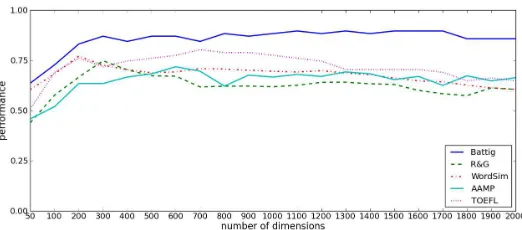
Figure 2: Behavioral evaluation of SVD models with range of dimensionality (see Section 3.1.1 for more details).
and Goodenough (1965) set of 65 concrete word pairs, and the strict-similarity subset of 203 pairs (Agirre et al., 2009) selected from the WordSim353 test-set (Finkelstein et al., 2002). Performance was evaluated with the Spearman correlation between the aggregate human judgements and pairwise cosine distances between word vectors in the model in question. Finally the TOEFL benchmark (Landauer and Dumais, 1997) consists of aggregate records from an examination task for learners of English, who have to identify a synonym among a set of distractors. Performance was measured as the percentage correct over 80 questions, if the cosine-distance of the target-synonym pair was smaller than the distance between the target and any of the distractor words.
For the NNSE and SVD models constructed here, an initial dimension setting of 300 was chosen, as this is in the middle range of those typically used in the literature. Where there was a choice with the other models we used the largest dimensionality available. For each of these two dimensionality reduction techniques, one model was constructed on the basis of document co-occurrences only (labelled “Doc” in the Figure 1), one using dependency co-occurrences only (“Dep”), and one using both sets of features combined (“Doc+Dep”).
From Ratinov et al. (2010) we took both the Collobert & Weston model (200 unscaled dimensions) and the HLBL model (100 scaled dimensions).2The LDA model was the default implementation included with the Gensim package ( ˇReh˚uˇrek and Sojka, 2010): an incremental algorithm based on Hoffman et al. (2010), over the English Wikipedia, using TF-IDF adjusted co-occurrences. As in clear from Figure 1 the SVD and NNSE models out-perform the other embeddings, though we cannot exclude that these models would be competitive with other parameter settings than those available, such as with a larger source corpus, or a different number of explanatory dimensions. Among the SVD and NNSE models, those based on dependency and combined (dependency and document) co-occurrences perform similarly well, and seem to have some advantage over document co-occurrences alone. And at this dimensionality setting SVD and NNSE seem similarly successful. As a result, in the subsequent analyses we concentrate on the combined SVD and combined NNSE models.
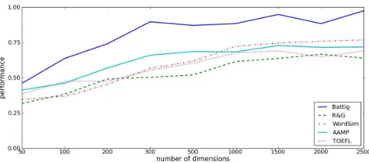
Figure 3: Behavioural evaluation of NNSE models with range of dimensionality (see Section 3.1.1 for more details).
We next examined how the choice of dimensionality affects the chosen SVD model (i.e., using both document and dependency co-occurrences) as evaluated with these behavioural tasks. As can be seen in Figure 2 performance peaks around the 200-300 dimension mark. In some tasks there is a fall-off in performance for higher dimensionalities, presumably as later dimensions are more noisy and/or irrelevant to these unsupervised tasks.
Finally we consider the effect of dimensionality for the NNSE models. In Figure 3 we see a very different pattern. For low dimensionalities it dramatically under-performs the SVD models, but at larger scales it continues to have an upward trend, peaking at similar levels.
In summary, these experiments demonstrate that NNSE and SVD models have similar peak perfor-mance, but with very different demands for dimensionality. NNSE needs at least 1000 dimensions to perform well, which may be understandable given that these dimensions must adequately describe all 40,000 words in the vocabulary used, and each word has on average 50 features active. The SVD model has very good performance at a dimensionality in the low hundreds, since it can pack information much more densely into a given number of features, and performance falls off as more noisy or irrelevant dimensions are added.
3.1.2 Neurosemantic Decoding Experiments
Mitchell et al. (2008) introduced a new task inneurosemantic decoding– using models of semantics to learn the mapping between concepts and the neural activity which they elicit during neuroimaging experiments. The dataset used here is that described in detail in Mitchell et al. (2008) and released publicly3in conjunction with the NAACL 2010 Workshop on Computational Neurolinguistics (Murphy et al., 2010). The Functional MRI (fMRI) data is from 9 participants while they performed a property generation task for each of 60 everyday concrete concepts: 5 exemplars of each of 12 semantic classes (mammals, body parts, buildings, building parts, clothes, furniture, insects, kitchen utensils, miscellaneous functional artifacts, work tools, vegetables, and vehicles). Each concept was presented six times and the resulting data-points were averaged to yield a single brain image for each concept, made up of approximately 20 thousand features (each a three-dimensional pixel, or “voxel”).
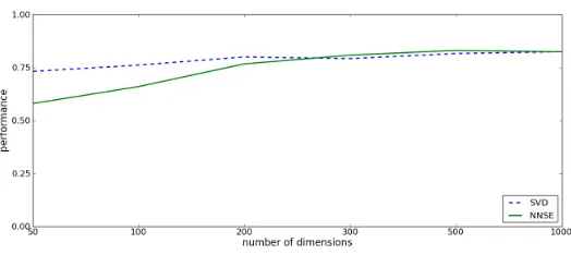
Figure 4: Neural activity test of NNSE and SVD models at range of dimensionalities (see Sec-tion 3.1.2 for details).
As in Mitchell et al. (2008), a linear regression model was used to learn the mapping from semantic features to brain activity levels. For each participant and selected fMRI feature we train a model to learn its activation as a regularised linear combination of the semantic features:
f=Cβ+λ||β||2 (5)
wheref is the vector of activations of a specific fMRI feature for different concepts, the matrixC contains the values of the semantic features for those concepts,βis the vector of weights we must
learn for each of those (corpus-derived) features, andλtunes the degree of regularisation.
The linear model was estimated with a least squared errors method andL2 regularisation, selecting the lambda parameter from the range 0.0001 to 5000 using Generalized Cross-Validation (see Hastie et al., 2011, p.244). The activation of each fMRI voxel in response to a new concept that was not in the training data was predicted by aβ-weighted sum of the values on each semantic dimension,
building a picture of expected the global neural activity response for an arbitrary concept. Again following Mitchell et al. (2008) we use a leave-2-out paradigm in which a linear model for each neural feature is trained in turn on all concepts minus 2, having selected the 500 most stable voxels in the training set using the same correlational measure across stimulus presentations. For each of the 2 left-out concepts, we predict the global neural activation pattern, as just described. We then try to correctly match the predicted and observed activations, by measuring the cosine distance between the model-generated estimate of fMRI activity and the that observed in the experiment. If the sum of the matched cosine distances is lower than the sum of the mismatched distances, we consider the prediction successful – otherwise as failed.
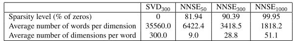
SVD300 NNSE50 NNSE300 NNSE1000 Sparsity level (% of zeros) 0 81.94 90.39 99.95 Average number of words per dimension 35560.0 6422.4 3418.5 1818.2 Average number of dimensions per word 300.0 9.0 28.8 51.1
Table 1: Comparison of sparsity level of SVD and NNSE models, the top 2 performing represen-tations in Section 3.1. Compared to the dense (non-sparse) SVD representation, NNSE results in significantly sparser embeddings than SVD.
3.2 Evaluating Level of Sparsity
In this section, we evaluate the sparsity of NNSE relative to the dense representations of SVD. The degree of sparsity in these two top-performing representations (Section 3.1) are compared in Table 1, for SVD atk=300, and for NNSE withk=50, 300, 1000. Given one such representation
A∈Rn×m, whereAi,:is the new embedding for theithword,sparsity levelmeasures the fraction of zero entries in this matrix out of the totaln×mentries.Average number of words per dimension
measures the average number of non-zero entries for each column ofA, where each column corresponds to one dimension. Average number of dimensions per wordcomputes the average number of non-zero entries for each row ofA, where each row is a representation for one word, as already mentioned above. We note that since SVD is a dense representation, varyingkin this case is not going to result in changes in the level of sparsity and values of the other two metrics compared in Table 1. Hence, in Table 1, we only present the results for SVD300for reference.
From Table 1, based on the sparsity level measurements, we observe that NNSE results in signifi-cantly sparser representations compared to the dense representation learned by SVD. We observe that askincreases, NNSE estimates even sparser representations. This might possibly be due to the fact that with a small number of available dimensions (e.g.,k=50), each dimension is used to
represent multiple latent concepts, resulting in non-zeros values for larger number of entries in each column and thereby in the full matrixA. In other words, each dimension acts as a mixture of latent concepts. However, we note that even at such settings (i.e.,k=50), NNSE achieves high sparsity
levels (81.9%) compared to the dense SVD.
From Table 1, we observe that askincreases, the average number of words per dimension decreases, from 6422.4 withk=50to 1818.2 withk=1000, i.e., each dimension becomes sparser as the number of available dimensions increases. This may be due to the fact, with smallerk(e.g.,k=50),
NNSE has to compress the input dataXinto a smaller number of dimensions, resulting in coarser granularity for each dimension.
Finally, from Table 1, we observe that askincreases, NNSE uses a larger number of dimensions per word, but even then, the resulting embeddings are significantly sparser compared to SVD, where each word is represented using all availablekdimensions.
3.3 Evaluating Interpretability
0 10 20 30 40 50 60 70 80 90 100
50 300 1000
[image:11.420.136.299.71.194.2]85.67 92.33 72 27.67 46.33 44
Interpretability Evaluation
P reci si o n Dimensions (k) SVD NNSEFigure 5: Comparison of interpretability of representations learned by SVD and NNSE for varying number of dimensions,k. Following (Boyd-Graber et al., 2009), word intrusion detection precision is used as the evaluation metric (higher precision implies higher interpretability). We observe that across all values of dimensionsk, NNSE results in significantly more interpretable representations than SVD. See Section 3.3 for details.
determine how coherent each column (dimension) ofAis.
Word Intrusion Detection Task: Following (Boyd-Graber et al., 2009), we use precision on a word intrusion detection task as the measure of coherence. The evaluation proceeds as follows: given a dimension (column)A:,j, we first reverse-sort the words based on membership values of those words in the column (i.e.,Ai,j,∀1≤i≤n). Next, we create a set consisting of the top 5 words from this ranked list, and also one word from the bottom half of this list, which is also present in the top 10th percentile of some other column inA. Thus, cardinality of this set is 6. The last word added from the bottom half is called anintruder. The goal is then to evaluate whether human subjects can identify this intruder word in a random ordering of the set. This process is repeated for each dimension, and the resulting precision is computed. This precision is used as the evaluation metric. Please note that we can compute precision in this setting as we know the true identity of the intruder word, it is just that this identity is hidden from the human evaluator. The idea behind this test is that if the current dimension is coherent, and thereby interpretable, then the human evaluator will be easily able to pick out the intruder word, thereby resulting in higher precision (higher is better). Example of such a set constructed from a dimension of the NNSE1000is shown below,
{bathroom, closet, attic, balcony, quickly, toilet}
wherequicklyis the intruder, as the rest of the words form a coherent set listing different parts of a house. Following (Boyd-Graber et al., 2009), this evaluation scheme is also known asreading tea leaves, where it was used to measure coherence of probabilistic topic models.
We use Amazon Mechanical Turk (MTurk)4to get human judgements in the word intrusion detection task. Given an embedding matrixA∈Rm×k, we constructednintruder sets as described above, one for each for thekdimensions. Fork>300, we randomly selected 300 dimensions for evaluation.
Model Top 5 Words (per dimension)
SVD300
well, long, if, year, watch plan, engine, e, rock, very get, no, features, music, via features, by, links, free, down works, sound, video, building, section
NNSE1000
inhibitor, inhibitors, antagonists, receptors, inhibition bristol, thames, southampton, brighton, poole delhi, india, bombay, chennai, madras
[image:12.420.84.322.69.180.2]pundits, forecasters, proponents, commentators, observers nosy, averse, leery, unsympathetic, snotty
Table 2: Examples of top 5 words for 5 randomly chosen dimensions from each of SVD300and NNSE1000. We observe that the dimensions in NNSE1000are much more semantically coherent (and thereby interpretable) compared to those in SVD300.
Detecting the intruding word in each such set was presented as a separate decision point, called Human Intelligence Task (HIT). Each HIT was evaluated by 3 different workers (turkers), and a compensation of $0.01 was provided for each feedback. Majority voting over the three responses was used as the final decision on a given set (HIT).
Discussion: Experimental results comparing precision of the SVD and NNSE representations on the word intrusion task for different value ofkare presented in Figure 5. From this figure, we observe that, for all values ofk, representations learned by NNSE are considerably more interpretable compared to those estimated by SVD. We find that interpretability for both of them peak atk=300. For qualitative comparison, top 5 words from 5 randomly selected dimensions each of SVD300and NNSE1000are presented in Table 2. From this, we get further anecdotal evidence about the higher interpretability of NNSE compared to SVD.
4 Related Work
Corpus-derived models of semantics have been extensively studied in the NLP and machine learning communities (Collobert and Weston, 2008; Ratinov et al., 2010; Turney and Pantel, 2010; Socher et al., 2011; Huang et al., 2012). Additionally, dimensionality reduction techniques such as SVD, and topic distributions learned by probabilistic topic models such LDA (Blei et al., 2003) can also be used to induce word embeddings. Although the embeddings learned by these methods have many overlapping properties, to the best of our knowledge, none of these previous proposals satisfy the three desirable properties: effective in practice, sparse, and interpretable. We find that Non-Negative Sparse Encoding (NNSE), a variation on a matrix factorization technique previously studied in the machine learning community, can result in semantic models which satisfy all three properties listed above.
Weight Top Words (per weighted dimension)
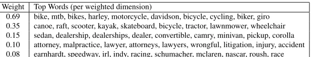
[image:13.420.64.377.70.128.2]0.69 bike, mtb, bikes, harley, motorcycle, davidson, bicycle, cycling, biker, giro 0.35 canoe, raft, scooter, kayak, skateboard, bicycle, tractor, lawnmower, wheelchair 0.15 sedan, dealership, dealerships, dealer, convertible, camry, minivan, pickup, corolla 0.10 attorney, malpractice, lawyer, attorneys, lawyers, wrongful, litigation, injury, accident 0.08 earnhardt, speedway, irl, indy, racing, schumacher, mclaren, nascar, roush, race
Table 3: Examples of top 5 weighted dimensions in NNSE for the tokenmotorbike, where each dimension is characterised by its top words.
Weight Top Words (per weighted dimension)
0.84 raspberry, peach, pear, mango, melon, strawberry, banana, berry, cranberry, citrus 0.25 peaches, apricots, pears, cherries, blueberries, figs, oranges, plums, raspberries 0.10 birch, fir, spruce, pine, elm, mahogany, aspen, cypress, willow, cedar
0.08 kreme, pillsbury, falafel, brownie, pretzel, pesto, horseradish, oreo, guacamole, pita 0.07 patties, slices, cubes, tacos, wedges, chunks, enchiladas, burritos, fajitas, tortillas
Table 4: Examples of top 5 weighted dimensions in NNSE for the tokenpear, where each dimension is characterised by its top words.
it can model human tasks that directly involve properties and their types, such as the feature norming exercises mentioned earlier (which our NNSE model is not capable of currently). Conversely, it has a disadvantage in that it does not address the ubiquitous synonymy and polysemy among property labels. For example, the Strudel representation formotorbikehas the properties (ordered by their strength of association):ride, rider, sidecar, park, road, helmet, collision, vehicle, car, moped. The corresponding representation in NNSE is dominated by the five dimensions listed in Table 3. For each dimension we show the words that characterize its meaning, and the magnitude of its contribution tomotorbike. These seem to describe the following respective classes which may correspond to topical usages of the word: (motor)cycling; leisure vehicles; vehicle sales; accidents and litigation; and racing. The corresponding listing forpearin Table 4, also exhibits some different senses of the word, coveringfruit,foodmore generally, andtrees.
Overall, we find that NNSE model is an alternative coding of the information stored in the SVD model. These models differ however in how that information is distributed across dimensions. The SVD model, as expected, is maximally compact, compressing as much information as possible into the minimum number of dimensions, but yielding individual dimensions that are very hard to interpret. The NNSE model is equally effective in modeling human judgements and brain activity elicited during lexical semantic tasks, but has a sparse structure which closely matches some common assumptions in cognitive science about conceptual representations.
5 Conclusion
which are effective in practice, sparse, and interpretable – a desirable list of properties which was not achievable by previously proposed methods.
There are still many ways in which we can extend and improve this new embedding method. First of all, we would like to test it as a component of core NLP tasks, such as chunking, named-entity-recognition, and parsing. We also plan to compare the individual NNSE dimensions to other benchmarks that explicitly cover categories and properties, such as feature norms, WordNet, and other collections of human judgements such as the 20Q data (Palatucci et al., 2009). Finally, we plan to look more closely at the relative contributions of different sources of input representations, such as dependency and document co-occurrences that underlie the current model, to examine the relationship between topical and attributional meanings that they correspond to.
Acknowledgments
We are thankful to Khaled El-Arini (CMU) and Min Xu (CMU) for many useful discussions on sparse coding. We thank Justin Betteridge (CMU) for his help with parsing the corpus, and Yahoo! for providing the M45 cluster over which the parsing was done. We also thank Marco Baroni (University of Trento) and Seshadri Sridharan (CMU) for assistance in preparing the behavioural benchmarks. We thank CMU’s Parallel Data Laboratory (PDL) for making the OpenCloud cluster available. We are thankful to the anonymous reviewers for their constructive comments. This research has been supported in part by DARPA (under contract number FA8750-09-C-0179), NIH (NICHD award 1R01HD075328-01), and Google. Any opinions, findings, conclusions and recommendations expressed in this paper are the authors’ and do not necessarily reflect those of the sponsors.
References
Agirre, E., Alfonseca, E., Hall, K., Kravalova, J., and Pas, M. (2009). A study on similarity and relatedness using distributional and WordNet-based approaches. Proceedings of NAACL-HLT 2009.
Almuhareb, A. and Poesio, M. (2004). Attribute-based and value-based clustering: An evaluation. InProceedings of EMNLP, pages 158–165.
Baroni, M. and Lenci, A. (2010). Distributional Memory: A General Framework for Corpus-Based Semantics.Computational Linguistics, 36(4):673–721.
Baroni, M., Murphy, B., Barbu, E., and Poesio, M. (2010). Strudel: A corpus-based semantic model based on properties and types.Cognitive Science, 34(2):222–254.
Battig, W. F. and Montague, W. E. (1969). Category Norms for Verbal Items in 56 Categories: A Replication and Extension of the Connecticut Category Norms. Journal of Experimental Psychology Monographs, 80(3):1–46.
Blei, D. M., Ng, A. Y., and Jordan, M. I. (2003). Latent Dirichlet Allocation.Journal of Machine Learning Research, 3(4-5):993–1022.
Boyd-Graber, J., Chang, J., Gerrish, S., Wang, C., and Blei, D. (2009). Reading tea leaves: How humans interpret topic models. InProceedings of the 23rd Annual Conference on Neural Information Processing Systems.
Bullinaria, J. A. and Levy, J. P. (2007). Extracting semantic representations from word co-occurrence statistics: A computational study.Behavior Research Methods, 39(3):510–526.
Callan, J. and Hoy, M. (2009). The ClueWeb09 Dataset.
Chen, S., Donoho, D., and Saunders, M. (2001). Atomic decomposition by basis pursuit.SIAM review, pages 129–159.
Collobert, R. and Weston, J. (2008). A unified architecture for natural language processing: Deep neural networks with multitask learning. InProceedings of the 25th international conference on Machine learning, pages 160–167. ACM.
Deerwester, S., Dumais, S., Furnas, G., Landauer, T., and Harshman, R. (1990). Indexing by latent semantic analysis.Journal of the American society for information science, 41(6):391–407.
Finkelstein, L., Gabrilovich, E., Matias, Y., Rivlin, E., Solan, Z., Wolfman, G., and Ruppin, E. (2002). Placing search in context: the concept revisited.ACM Transactions on Information Systems, 20(1):116–131.
Garrard, P., Lambon Ralph, M. A., Hodges, J. R., and Patterson, K. (2001). Prototypicality, distinctiveness, and intercorrelation: Analyses of the semantic attributes of living and nonliving concepts.Cognitive Neuropsychology, 18(2):25–174.
Griffiths, T. L., Steyvers, M., and Tenenbaum, J. B. (2007). Topics in semantic representation.
Psychological Review, 114(2):211–244.
Hall, J., Nilsson, J., Nivre, J., Eryigit, G., Megyesi, B., Nilsson, M., and Saers, M. (2007). Single Malt or Blended? A Study in Multilingual Parser Optimization.Proceedings of CoNLL Shared Task Session, pages 933–939.
Hastie, T., Tibshirani, R., and Friedman, J. (2011).The Elements of Statistical Learning, volume 18 ofSpringer Series in Statistics. Springer, 5th edition.
Hoffman, M. D., Blei, D. M., and Bach, F. (2010). Online Learning for Latent Dirichlet Allocation. In Lafferty, J., Williams, C. K. I., Shawe-Taylor, J., Zemel, R. S., and Culotta, A., editors,
Proceedings of NIPS.
Hoyer, P. O. (2002). Non-negative sparse coding. InProceedings of the 12th IEEE Workshop on Neural Networks for Signal Processing, pages 557–565. Ieee.
Huang, E., Socher, R., Manning, C., and Ng, A. (2012). Improving word representations via global context and multiple word prototypes. InProceedings of ACL.
Jones, E., Oliphant, T., Peterson, P., and Et Al. (2001). SciPy: Open source scientific tools for Python.
Karypis, G. (2003). CLUTO: A Clustering Toolkit. Technical Report 02-017, Department of Computer Science, University of Minnesota.
Lehoucq, R. B., Sorensen, D. C., and Yang, C. (1998).Arpack users’ guide: Solution of large scale eigenvalue problems with implicitly restarted Arnoldi methods. SIAM.
Levy, J. P. and Bullinaria, J. A. (2012). Using Enriched Semantic Representations in Predictions of Human Brain Activity.Proceedings of the 12th Neural Computation and Psychology Workshop, pages 292–308.
Lin, D. (1998). Automatic Retrieval and Clustering of Similar Words. InProceedings of COLING-ACL, pages 768–774.
Lund, K. and Burgess, C. (1996). Producing high-dimensional semantic spaces from lexical co-occurrence.Behavior Research Methods, Instruments, and Computers, 28:203–208.
Lund, K., Burgess, C., and Atchley, R. (1995). Semantic and associative priming in high di-mensional semantic space. InProceedings of the 17th Cognitive Science Society Meeting, pages 660–665.
Mairal, J., Bach, F., Ponce, J., and Sapiro, G. (2010). Online learning for matrix factorization and sparse coding.The Journal of Machine Learning Research, 11:19–60.
McRae, K., Cree, G. S., Seidenberg, M. S., and McNorgan, C. (2005). Semantic feature production norms for a large set of living and nonliving things.Behavior Research Methods, Instruments, & Computers, 37(4):547–559.
Miller, G. A., Beckwith, R., Fellbaum, C., Gross, D., and Miller, K. (1990). Introduction to WordNet: an on-line lexical database.International Journal of Lexicography, 3(4):235–244.
Mitchell, T. M., Shinkareva, S. V., Carlson, A., Chang, K.-M., Malave, V. L., Mason, R. A., and Just, M. A. (2008). Predicting Human Brain Activity Associated with the Meanings of Nouns.
Science, 320:1191–1195.
Murphy, B., Korhonen, A., and Chang, K. K.-M., editors (2010).Proceedings of the 1st Workshop on Computational Neurolinguistics, NAACL-HLT, Los Angeles. ACL.
Murphy, B., Talukdar, P., and Mitchell, T. (2012). Selecting Corpus-Semantic Models for Neu-rolinguistic Decoding. InProceedings of *SEM-2012.
Murphy, G. (2004).The big book of concepts. MIT Press.
Nancy Ide and Keith Suderman (2006). The American National Corpus First Release.Proceedings of the 5th LREC.
Nation, P. and Waring, R. (1997). Vocabulary size, text coverage and word lists. In Schmitt, N. and McCarthy, M., editors,Vocabulary Description acquisition and pedagogy, pages 6–19. Cambridge University Press.
Padó, S. and Lapata, M. (2007). Dependency-based construction of semantic space models.
Computational Linguistics, 33(2):161–199.
Rapp, R. (2003). Word Sense Discovery Based on Sense Descriptor Dissimilarity.Proceedings of the Ninth Machine Translation Summit, pp:315–322.
Ratinov, L., Turian, J., and Bengio, Y. (2010). Word representations: a simple and general method for semi-supervised learning.Proceedings of the 48th ACL, 96(July):384–394.
ˇReh˚uˇrek, R. and Sojka, P. (2010). Software Framework for Topic Modelling with Large Corpora. InProceedings of New Challenges Workshop, LREC 2010, pages 45–50. ELRA.
Rubenstein, H. and Goodenough, J. B. (1965). Contextual correlates of synonymy. Communica-tions of the ACM, 8(10):627–633.
Sahlgren, M. (2006).The Word-Space Model: Using distributional analysis to represent syntag-matic and paradigsyntag-matic relations between words in high-dimensional vector spaces. Dissertation, Stockholm University.
Schunn, C. D. (1999). The Presence and Absence of Category Knowledge in LSA. InProceedings of the 21st Annual Conference of the Cognitive Science Society., Mahwah. Erlbaum.
Schütze, H. and Pedersen, J. (1993). A Vector Model for syntagmatic and paradigmatic relatedness. InMaking Sense of Words Proceedings of the 9th Annual Conference of the University of Waterloo Centre for the New OED and Text Research, pages 104–113.
Socher, R., Huang, E., Pennington, J., Ng, A., and Manning, C. (2011). Dynamic pooling and unfolding recursive autoencoders for paraphrase detection. Advances in Neural Information Processing Systems, 24.
Turney, P. D. and Pantel, P. (2010). From Frequency to Meaning: Vector Space Models of Semantics.Artificial Intelligence, 37(1):141–188.