www.nat-hazards-earth-syst-sci.net/8/1067/2008/ © Author(s) 2008. This work is distributed under the Creative Commons Attribution 3.0 License.
and Earth
System Sciences
Optimal design under uncertainty of a passive defense structure
against snow avalanches: from a general Bayesian framework to a
simple analytical model
N. Eckert1, E. Parent2, T. Faug1, and M. Naaim1
1UR ETNA, Cemagref Grenoble, BP 76, 38 402 Saint Martin d’H`eres, France
2Equipe MORSE, UMR 518 AgroParisTech/INRA, 19 avenue du Maine, 75732 Paris cedex 15, France
Received: 26 March 2008 – Revised: 8 August 2008 – Accepted: 30 August 2008 – Published: 15 October 2008
Abstract. For snow avalanches, passive defense structures are generally designed by considering high return period events. In this paper, taking inspiration from other natural hazards, an alternative method based on the maximization of the economic benefit of the defense structure is proposed. A general Bayesian framework is described first. Special atten-tion is given to the problem of taking the poor local informa-tion into account in the decision-making process. Therefore, simplifying assumptions are made. The avalanche hazard is represented by a Peak Over Threshold (POT) model. The in-fluence of the dam is quantified in terms of runout distance reduction with a simple relation derived from small-scale ex-periments using granular media. The costs corresponding to dam construction and the damage to the element at risk are roughly evaluated for each dam height-hazard value pair, with damage evaluation corresponding to the maximal ex-pected loss. Both the classical and the Bayesian risk func-tions can then be computed analytically. The results are illus-trated with a case study from the French avalanche database. A sensitivity analysis is performed and modelling assump-tions are discussed in addition to possible further develop-ments.
Correspondence to: N. Eckert ([email protected])
1 Introduction
Mitigation against natural hazards traditionally involves computing high return period events for the design of defense structures (Ancey et al., 2004; Eckert et al., 2007). Nowa-days such methods are strongly contested in fields such as hydrology (Krzysztofowicz, 1983; Bernier, 2003) and engi-neering (Jordaan, 2005) by economic approaches that aim at optimizing the use of public funds. Their principle is to choose the design value that minimizes the expected loss. The model describing the stochasticity of the phenomenon is therefore combined with a utility function and then the expected loss associated with each value of the decisional variable is computed. Technical difficulties are overcome as a result of important methodological developments concern-ing simulation-based algorithms (M¨uller, 1999; Amzal et al., 2006).
loss in case of an extreme avalanche can greatly increase if a slight increase in the runout area is considered. On the other hand, when the optimization of a defense structure is car-ried out with respect to a given scenario, the retained defense structure is obviously more efficient if this scenario occurs than if the optimum computed by averaging all over the haz-ard distribution is retained.
Risk computations have also been performed in the avalanche field, but mainly for hazard mapping purposes (Keylock et al., 1999; Chernouss and Fedorenko, 2001; Bar-bolini et al., 2004a; Grˆet-Regamey and Straub, 2006); most authors use the annual probability of being killed by an avalanche as a definition of risk. This type of method is in-cluded in the current legislation in Iceland (Jonasson et al., 1999, Arnalds et al., 2004).
This paper illustrates the potential of a decision theoreti-cal framework for the design of a passive avalanche defense structure, i.e. a defense structure that does not decrease the avalanche release probability but reduces the damage to the elements at risk. More precisely, we focus on the case of a vertical dam protecting one or several buildings situated at a known position on the avalanche path. Critical points by comparison with hydraulics are as follows: (i) the local infor-mation available for avalanche studies is generally poor. In addition, because of the complex nature of the flowing fluid (Dent and Lang, 1980; Bouchet et al., 2004), (ii) the evalu-ation of the influence of the dam on the flow in the runout zone where the elements at risk are situated is not easy, and (iii) complex hazard models are generally used (Har-bitz et al., 1998), making stochastic approaches too time-consuming for operational purposes. Problem (i) is treated within a Bayesian framework (Krzysztofowicz, 2001; Girard and Parent, 2004; Clark, 2005) that allows uncertainty due to the lack of local information being processed up to the decision. Problem (ii) is addressed by incorporating a semi-empirical formulation of the dam’s influence into the stochas-tic avalanche model. Problem (iii) is overcome by consider-ing simplifyconsider-ing assumptions for the quantification of both the hazard and the cost evaluation, so that the risk computations can be performed analytically.
Section 2 briefly presents the elementary bricks that are needed for the Bayesian optimal design of an avalanche dam. Section 3 proposes strong assumptions and puts the bricks together, so as to obtain the analytical expression of the risk functions. Section 4 applies the model obtained to a real case study from the French avalanche database. Section 5 dis-cusses the results with special attention devoted to modelling assumptions and possible further developments. Section 6 offers a general conclusion highlighting the relevance of the decisional model for real case applications.
2 Materials and methods
2.1 Hazard model and associated uncertainty
For convenience, the avalanche is assumed to move along a curvilinear two-dimensional profile whose equation in a Cartesian frame isz=f (x), wherezis the altitude andxthe distance measured along a horizontal axis starting at the top of the path and following the avalanche thalweg. A distinc-tion is made between avalanche magnitudeyand avalanche frequencya. Avalanche magnitude includes all the quan-titative characteristics that vary from one event to another: runout distance, velocity and pressure profiles, snow vol-ume, etc. Avalanche frequency is the number of avalanches recorded during a given winter. The stochastic hazard model is noted l (y, a|θM, θF), indicating that the joint
distribu-tion l of the random numbers y and a is indexed by the parameters θM, θF. Finally, the hypothesis of
magnitude-frequency independence is made, considering that the num-ber of avalanches per winter does not affect their quantitative characteristics (Eq. 1). This classical hypothesis in avalanche modelling is fulfilled if the number of avalanches affecting the studied path each winter is not too high (Eckert et al., 2008a).
l (y, a|θM, θF)=l (y|θM)×l (a|θF) (1)
The typical inference challenge is to obtain point estimates ∧
θM,
∧
θF for the parametersθM, θF knowing the data available
on the studied site in order to use them in a predictive phase for quantifying reference hazards and/or designing defense structures. However, obtaining point estimates such as maxi-mum likelihood point estimates can be very tricky depending on the model considered. Moreover, if data quantity is small, which is usually the case in avalanche studies, such point es-timates are highly uncertain. They therefore cannot be used for prediction with a good level of confidence, and rigorous engineering practices should take into account this lack of information on the model’s parameters. Bayesian inference (Bayes, 1763) is appropriate, offering a fair quantification of the state of knowledge given the data through the posterior distributionp (θM, θF|data). Its computation is carried out
by processing the model using Bayes theorem (Eq. 2) at the cost of the specification of a prior distributionπ (θM, θF).
p (θM, θF|data)∝l (y, a|θM, θF)×π (θM, θF) (2)
2.2 Cost quantification and risk computation
Let us assume that one building is situated at the abscissaxb
of the runout zone. The construction of a vertical protective dam at the abscissaxd is envisaged and the problem is to
choose the dam heighthdthat minimizes economic losses.
The cost functionC (hd, y, a)is the basic tool for a
y, a). A general additive form for the cost function is given by Eq. 3. The first termCo(hd)quantifies the cost of
con-structing a dam of heighthd. C1(hd, yt k)is the cost of the
damage inflicted by the avalanche k ∈ [1, at] of the year
t ∈ [1,+∞[ given that the dam height is hd and that at
avalanches have been observed during the wintert. This cost has to be actualized, assuming a known annual interest rate itfor the yeart. The second term of Eq. 3 therefore quantifies
the total damage inflicted on the building by the successive snow avalanches that occur starting at the time of the dam construction. Note that the damage caused to the dam by the successive avalanches is not explicitly taken into account in this formula (see Sect. 5.3 for discussion).
Under the strong hypothesis of stationarity, all theyt k’s
are identically distributed. In addition, under the magnitude-frequency independence hypothesis, the total cost depends on the expected number of avalanchesE[a] only. The cost function can therefore be considerably simplified (Eq. 4), with a total actualization rateAdepending on the annual in-terest rates only (Eq. 5).
C (hd, y, a)=Co(hd)+
+∞
X
t=1
at X
k=1
1 (1+it)t
×C1(hd, yt k) (3)
C (hd, y, a)=Co(hd)+A×E[a]×C1(hd, y) (4)
A=A(i)=
+∞
X
t=1
1 (1+it)t
(5)
For an easy quantification of the pertinence of the decision, a reference state has to be introduced. We define the utility functionu (hd, y, a)as the cost difference for a given
haz-ard value between the construction of a dam of heighthdand
no dam (Eq. 6). Note that in the general decision theoretical framework, the utility function generally has a more specific definition including the behavior of the decision maker man-aging risk. We assume here that the decision maker behaves neutrally toward risk, which should be the case if substantial public funds are involved.
u (hd, y, a)=Co(hd)+A×E[a]×(C1(hd, y)−C1(0, y)) (6) The expected utility is known as the classical risk RC(hd, θM, θF). It is a function of the decisional variable
hd and the parametersθM, θF describing the hazard model
(Eq. 7). It quantifies the mean economic loss that must be expected if an obstaclehdis constructed instead of
maintain-ing the existmaintain-ing situation. More simply, it is the opposite of the expected economic benefit of the dam construction. With the utility model proposed, only the integration over the mag-nitude variability is necessary (Eq. 8). According to the clas-sical risk setting, the optimal dam heighth∗C minimizes the expected utility and is obtained by solving Eq. 9. Note that, in all computations performed in this paper, thish∗Cis the ef-fective height seen by the incoming avalanche. For practical
purposes, the mean depth of the snow cover has therefore to be added.
RC(hd, θM, θF)=Ey,a[u (hd, y, a)] (7)
RC(hd, θM, θF)=Co(hd)+
AE[a|θF]
Z
(C1(hd, y)−C1(0, y)) l (y|θM)dy (8)
∂RC
hd,
∧ θM,
∧ θF
∂hd
=0 (9)
Obviously, the solution of Eq. 9 is a function of the pa-rameters θM, θF. Current engineering practice is to plug
point estimates ∧ θM,
∧
θF intoRC(hd, θM, θF)and to
recom-mendh∗C=h∗C ∧
θM,
∧ θF
. The classical optimal design pro-cedure therefore assumes perfect knowledge of the avalanche model’s parameters. However, disconnecting the statistical problem from the decisional problem may have undesirable consequences. Indeed, the decisional problem is then treated as if the hazard parameters were perfectly known, which is unrealistic with poor local information. Moreover, the classical risk setting does not account for a discrepancy be-tween the statisticians’s and decision maker’s points of view when inferring model parameters. The statistician generally searches for point estimates minimizing a variance criterion, which is a symmetrical quadratic function. On the contrary, decision makers may consider nonsymmetrical cost func-tions since overestimating the design value is obviously more acceptable than underestimating it.
The Bayesian risk RB(hd)takes into account the
addi-tional uncertainty affecting the hazard by averaging through-out the posterior distribution of the parameters (Eq. 10), clearly incorporating the estimation error into the decisional process. The Bayesian risk can therefore be seen as a function ofhd only, which makes it easy to determine the
Bayesian optimal heighth∗B (Eq. 11). Obviously, it is also a function of the prior knowledge and of the data used for inference.
RB(hd)=EθM,θF[RC(hd, θM, θF)]= Z
RC(hd, θM, θF) p (θM, θF|data) dθMdθF (10)
h∗B =Argmin
hd
(RB(hd)) (11)
2.3 Linear model for obstacle effects
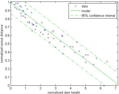
Fig. 1. Influence of the dam: model versus experimental data.
α=0.1376±0.006. Raw data measured in Davos, Bristol and Reyk-javik are available in Hakonardottir et al. (2001). Raw data mea-sured in Grenoble and Bologna are available in Faug et al. (2003).
on important research using full-scale experiments (Lied et al., 2001) and small-scale experiments (Faug, 2004) as well as numerical modeling (Naaim et al., 2004). The extensive literature on this topic is reviewed by Faug et al. (2008). For instance, converging results have been obtained while study-ing the influence of a vertical dam on a so-called reference hazard, a given avalanche defined by its flow depth, runout distance, longitudinal velocity profile, etc.
More precisely, a first-order development of the energy dissipation induced by a dam assuming a punctual “black box” effect on the flow gives a linear relationship between the runout distance reduction and the ratio between the dam height hd and the depth of the reference flow without the
damho (Faug et al., 2008). The reference runout distance
xstopo is therefore reduced toxstop(hd), with a proportional-ity coefficientαquantifying the dissipation power of the dam (Eq. 12). The theoretical relationship is largely supported by several small-scale experiments on rapid granular avalanches with typical Froude numbers higher than 2–3 (H´akonard´ottir et al., 2001; Faug et al., 2003). Figure 1, for instance, shows good agreement between the model and experimental data, with nearly all the observations falling into the 95% confi-dence interval. Moreover, these results are compatible with recent analysis of full-scale snow avalanches overflowing a dam that shows a linear scaling betweenxstop(hd)and hd
(Gauer and Kristensen, 2005; Faug et al., 2008). The pro-portionality coefficient α is known to be around 0.14 for dry granular materials modelling dry dense avalanches (see Sect. 5.2 for discussion and Sect. 4.4.4 for a sensitivity anal-ysis).
xstop(hd)−xd
xstopo−xd
=1−α×hd ho
(12)
Obviously, the semi-analytical relation of Eq. 12 has a number of limitations. The most obvious ones are xstop(hd)−xd>0 andhd<ho×1α, since for higher dams the
avalanche flow is fully stopped andxstop(hobs)−xd drops to
zero. Other limitations related to the flow regime will be dis-cussed in Sect. 5.2.
Finally, it is important to mention that the reference runout xstopo and the reference flow depth ho were unknown for the full-scale observations of avalanches overtopping dams, which did not allow verifying Eq. 12 and consequently esti-mating the value ofαon real avalanches. The value chosen forαis thereby the value obtained from the rapid laboratory granular avalanches. Sufficient knowledge is assumed forα by settingα=α∧=0.1376 for all the computations. This latter hypothesis is discussed in Sect. 4.4.4.
3 A simple analytical risk model
3.1 A conjugate POT model for monovariate avalanche hazard
Quantifying avalanche hazard generally involves multivari-ate modelling of avalanche magnitude to account for at least runout distance, flow depth and pressure variations in the runout zone. Nevertheless, avalanche magnitude is limited in this paper to runout distance, i.e., the most critical value for avalanche hazard mapping. Moreover, the runout distances exceeding the dam abscissa without a dam are assumed to be exponentially distributed (Eq. 13), so thaty=xstopo,θM=ρ.
More classically, the number of exceedences occurring dur-ing a given winter is assumed to be Poisson-distributed (Eq. 14), so thatθF=λ. The mathematical expectation of the
frequency model used in the cost function is then simply the parameterλ. The runout abscissaxstopTcorresponding to any
return periodT can be easily computed (Eq. 15). This very simple hazard model with two parameters only(ρ, λ)is well known in hydrology (Parent and Bernier, 2003) as a Peak Over Threshold (POT) model (Coles, 2001). Its relevance in the field of snow avalanches is discussed in Sect. 5.1. l xstopo
ρ, xstopo>xd
=ρ×exp −ρ× xstopo−xd
(13)
l (a|λ )= λ
a
a! ×exp(−λ) (14)
xstopT =
1
ρ ×ln(λT )+xd (15)
The analytical computation of the posterior distribution of the parameters ρ, λ is possible with hypotheses for math-ematical convenience. Conjugate Gamma priors are cho-sen for both parameters of the hazard model with two pairs aρ, bρand(aλ, bλ)to be specified (e.g., Eq. 16). Marginal
the data. More precisely, with a data set ofn avalanches exceeding the thresholdxd inmyears andS(n)the sum of
these exceedences,aλ0=aλ+m,bλ0=bλ+n,aρ0=aρ+S(n)and
bρ0=bρ+n. Whennandmare large enough, the prior
knowl-edge does not play much of a role. This is especially true if poorly informative priors (Bernardo and Smith, 1994) are chosen. This will be the case in this paper, so that classi-cal and Bayesian inferences asymptoticlassi-cally lead to the same estimators (Berger, 1985).
π ρaρ, bρ=
abρρ
0 bρ
×ρbρ−1×exp −a
ρ×ρ (16)
3.2 Simplified cost and utility functions
Starting from Eq. 4, two additional assumptions are made. First, the construction cost is assumed to increase linearly with dam height. Second, the damage caused to the build-ing by a snow avalanche is assumed to depend only on runout distance, with the damage term simply modeled by the product of an indicator function with the economic value of the buildings. The indicator function I{xstop(hd)≥xb}=1 ifxstop(hd)≥xb andI{xstop(hd)≥xb}=0 if xstop(hd)<xb. The damage is therefore maximal as soon as the building is at-tained, whereas the building remains obviously undamaged if the avalanche does not reach its abscissa (Eq. 17). This is obviously a very rough approximation, but consistent with the simplifications also made for the modelling of hazard and dam influence. Though, more elaborate formulations have been recently proposed (e.g. Barbolini et al., 2004b), but the related uncertainty is still very high. See Sect. 5.3.2 for dis-cussion.
C hd, xstop(hd) , a=Cohd+AλC1I{xstop(hd)≥xb} (17) Combining Eq. 17 and the influence of the dam on runout distances (Eq. 6), the cost corresponding to the runout dis-tancexstop(hd)can be expressed using only the reference
flow ho and the reference runout distance xstopo (Eq. 18).
The corresponding utility function is then easily obtained us-ing the properties of indicator functions (Eq. 19). Equation 19 establishes that the dam is useful only for avalanches that flow beyond the building without the dam but are stopped before the building with the dam.
C hd, xstopo, a
=Cohd+AλC1In
(xstopo−xd)
1−αhdho≥xb−xd o (18)
u hd, xstopo, a=Cohd+AλC1I
xb−xd
1−αhd
ho
+xd≤xstopo<xb
(19)
3.3 Analytical risk computations
The analytical integration of the utility function throughout the hazard model is possible (Eq. 20), with a change of vari-ables in the integral easily leading the result (Eq. 21). The risk function obtained depends on the dam height and the two parameters of the hazard model.
RC(hd, ρ, λ)=Cohd+
AλC1
xb Z
xb−xd
1−αhdho +xd
ρexp −ρ xstopo−xd
dxstopo (20)
RC(hd, ρ, λ)=Cohd+
AλC1 exp
−ρ (xb−xd)
1−αhd
ho !
−exp(−ρ (xb−xd))
!
(21)
The Bayesian risk is the mathematical expectation of the classical risk over the joint posterior distribution of the pair (ρ, λ)(Eq. 22). Given the model’s properties, the joint pos-terior distribution of the pair (ρ, λ) is simply the product of their marginal posterior distributions. The integral over λis the mathematical expectation of a Gamma distribution. Moreover, the properties of summation to 1 of a probabil-ity distribution can be used to compute the integral overρ (Eq. 23).
RB(hd)=Cohd+AC1 Z ∞
λ=0
λ× ∞
Z
ρ=0
exp −ρ (xb−xd) 1−αhd
ho
!
−exp(−ρ (xb−xd))
!
p (λ, ρ|data) dρdλ
(22)
RB(hd)=Cohd+
AC1 b0λ a0λ
a0ρ a0
ρ+ xb−xd 1−αhdho
bρ0
− a
0
ρ
a0
ρ+xb−xd
!b0ρ
(23)
Unfortunately, the analytical optimization of Eqs. 21 and 23 cannot be performed, but the numerical determination of the dam heights that minimize both risk functions is easy.
4 Application to a case study
4.1 Case study presentation
Fig. 2. Case study: topography and available historical data.
Town-ship of Bessans, Savoie, France.
Table 1. Main characteristics of the case study.
Real case study
Max altitude (m) 2850 Min altitude (m) 1675 Total drop (m) 1175 Total length (m) 1763 Mean slope (deg) 38.2 dam abscissa (m) 1550 dam altitude (m) 1704 Number of years of survey 31 Number of exceedances 28
2004). It is situated in the township of Bessans, in the Savoie department. It is 1763 m long from its top to the Arc River, with a vertical drop of 1175 m (Fig. 2). It is only very slightly channeled and the average slope is steep (Table 1). Several concavity changes that would make numerical mod-elling (Naaim et al., 2004) of the flow difficult occur along the slope’s profile. However, the runout zone that consists in the gentle slope preceding the Arc River (x=1763 m) is rather regular, making the use of a simple stochastic model for runout distances possible.
An exposed building is assumed to be situated in the runout zone. It seems unrealistic to consider a building at an abscissa corresponding to a return period of less than 10 years. In addition, an upper limit for zoning restrictions less than 1000 years is always adopted. Consequently, only build-ings implanted at abscissasxb corresponding to return
peri-ods ranging from 10 to 1000 years are investigated, with spe-cial attention paid to the well-known return periods of 30, 100 and 300 years (Ancey and Richard 2000; Bardou, 2006). The position of the dam to be designed is fixed at an ab-scissa theoretically corresponding to the beginning of the runout zone. In the avalanche field, the engineering practice
Fig. 3. Frequency model. Data versus model givenλ=∧λ(left) and posterior distribution of the parameter (right).
initiated by Salm et al. (1990) considers that the runout zone begins where the local slope decreases under 10◦. When applied to this path, this empirical rule impliesxd=1550 m.
Note that in reality some avalanches have on this path stopped on steeper slopes (Fig. 2), but they are of no rele-vance for risk assessment as their runout distances are very short.
During the 1973–2003 time period, 28 avalanches exceed-ingxdwere recorded by the local forestry service. The most
extreme runout distance recorded corresponds to the Arc River, but beyond it, the terrain remains rather flat, making it possible for extreme avalanches to reach higher abscissas. 4.2 Bayesian inference of the POT model
Poorly informative priors are used, aλ=aρ=0.001 and
bλ=bρ=0.01, respectively, so that a0λ=31.001, b
0
λ=28.01,
aρ0=1208.7 and b0ρ=28.01. Figures 3 and 4 illustrate the posterior Gamma distributions of model parameters as well as a comparison between the data and the model. The pos-terior distributions of both parameters are nicely shaped, with a variance much lower than for the prior distribu-tions, which reflects the amount of information conveyed by the data. Bayesian estimators of the model’s parame-ters equal the posterior means under the assumption of a quadratic loss function, i.e.,Ea0
λ,b 0 λ[λ]=
∧ λ=b
0 λ
a0 λ
=0.9035 and Ea0
ρ,b0ρ[ρ]= ∧ ρ=b
0 ρ
a0 ρ
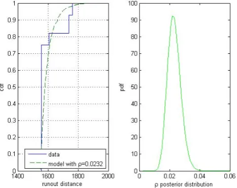
Fig. 4. Magnitude model. Data versus model givenρ=∧ρ(left) and posterior distribution of the parameter (right).
The frequency model givenλ=∧λis very close to the ob-served avalanche activity, which indicates that a Poisson model describes the randomness of the number of excee-dences well (Fig. 3). The adequacy between the data and the magnitude model givenρ=ρ∧ is less satisfactory, with the empirical distribution being strongly discrete. A part of this discrepancy can be attributed to the strong dependency of runout distance distribution on local topography, which makes many avalanches stop at abscissas corresponding to a significant decrease in the local slope. Nevertheless, a large part of this discrepancy is also caused by observation errors: only runout altitudes are recorded in the French avalanche database, so that runout abscissas are not actually observed and have to be recomputed using the topographic relation-shipz=f (x). For avalanches that stop on the valley floor, this topographic relationship is obviously poorly defined, so that the true distribution of runout distances is probably less discrete than suggested by the raw observations.
4.3 Optimal design 4.3.1 Parameterization
For both cost and utility functions, the depth of the refer-ence flow is necessary. However, it is not modelled with a monovariate POT model and therefore has to be consid-ered as constant from one avalanche to another (see Sect. 5.1 for discussion). For simplicity and to cope for the available information, a mean reference flow ho=1 m was assumed.
This implieshd<α1=7.15 m for the relationship describing
the influence of the dam to be valid. Another solution would have been to compute the flow depth corresponding to each past event from the deposit volumes (e.g. Meunier et al.,
Fig. 5. Classical and Bayesian risk functions for a building situated
at a 100-year return period abscissa.λ=0.9035 andρ=0.0232 for the classical risk. a0λ=31.001,bλ0=28.01,a0ρ=1208.7 andb0ρ=28.01 for the Bayesian risk.Co=5530 C .m−1,C1=300 000 C,α=0.1376,
ho=1 m andA=25.
Table 2. Classical and Bayesian optimal heights for buildings
situ-ated at abscissas corresponding to different return periods.
T10 T30 T100 T300 T1000
xstopT 1645.7 1693.1 1745.1 1792.5 1844.4
h∗C(m) 5.42 4.32 3.02 1.77 0.34
h∗B(m) 5.69 4.73 3.58 2.47 1.19
δh∗=h∗B−h∗C(m) 0.27 0.41 0.56 0.7 0.85
δh∗(%) 5 9.5 18.5 39.6 250
2004). Other numerical values used are Co=5530 C m−1,
C1= C 300 000 and a constant annual interest rate of 4%.
Construction and damage costs correspond to a small dam and to a nice single house, whereas A=
+∞
P
t=1 1
(1+0.04)t is
equivalent to 25 years.
4.3.2 Classical risk for a building situated at a 100-year runout abscissa
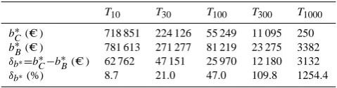
Table 3. Expected benefit of the optimal dam construction for
build-ings situated at abscissas corresponding to different return periods, classical and Bayesian computations.
T10 T30 T100 T300 T1000
bC∗ ( C ) 718 851 224 126 55 249 11 095 250
bB∗ ( C ) 781 613 271 277 81 219 23 275 3382
δb∗=b∗C−b∗B( C ) 62 762 47 151 25 970 12 180 3132
δb∗(%) 8.7 21.0 47.0 109.8 1254.4
C 55 000 at the optimal height. For higher dams, the eco-nomic benefit decreases again, indicating that the additional protective effect no longer compensates the additional con-struction cost. For high dams, the risk function tends to increase linearly with the dam height according to the cost function chosen. Note that the obtained optimal height may appear very small with regards to the size of the avalanche path. But this height is a direct consequence of the chosen building value and building position. Indeed, a single house with no inhabitants attained by a centennial avalanche only is considered, so that it cannot be economically justified to build a higher dam.
4.3.3 Bayesian risk for a building situated at a 100-year runout abscissa
Figure 5 also shows the corresponding Bayesian risk func-tion. The Bayesian risk function is relatively close to the classical risk function in terms of shape and value. Neverthe-less the Bayesian optimal height (3.58 m) is slightly higher than the classical optimal height (3.02 m), with a relative dif-ference of 18.5%. Moreover, the benefit expected from the construction of the optimal dam is higher when the Bayesian computation is used ( C 81 219) than when the classical com-putation is used ( C 55 249).
These effects should be attributed to the explicit incorpo-ration of hazard uncertainty into the decisional process. Us-ing the posterior distribution of hazard parameters instead of point estimates adds estimation error to the variability of the natural process. This is especially critical for the extreme events that attain high return period abscissas such as the 100-year return period abscissa and justify the dam construc-tion. It is therefore understandable that an additional protec-tion effort appears as economically advantageous when pa-rameter uncertainty is taken into account for the decision.
It can also be noted that the risk function around the op-timum is flatter for the Bayesian risk than for the classical risk, indicating that a large range of dam heights corresponds to very close risk values. This is due to the smoothing effect of averaging over the posterior distribution of the model’s parameters. It reflects the poor lever of local information fairly well and should therefore not be seen as a drawback of choosing the Bayesian framework instead of the classical
one. Moreover, from a more practical point of view, it can also be argued that different choices with different trade-offs between investment and protection corresponding roughly to a similar economic efficiency are then possible, giving more latitude for a political decision.
Note that poorly informative priors were used for the com-putation of the Bayesian risk function, so that both risk func-tions contain the same information and can be compared. For instance, the difference between the two optima is at-tributable to the lack of local knowledge only, and not to the influence of the priors. For an engineering project, informa-tive priors can be used if available, but then, an additional sensitivity analysis is required.
4.4 Sensitivity analysis
As the analytical expressions of both classical and Bayesian risk functions are available, a full sensitivity analysis to the choice of the different numerical values can easily be con-ducted. In addition to parameter uncertainty, different factors can be investigated: hazard magnitude, hazard frequency, po-sition of the building and costs. Illustrations are provided in this section using mainly Bayesian risks, but the same con-clusions hold for classical risks, with alwaysh∗B≥h∗C. 4.4.1 Hazard magnitude and position of the buildings The risk function depends on the combination of hazard mag-nitude with the distance between the buildings and the dam, i.e., the productρ×(xb−xd)for the classical risk function
and the sumaρ0+xb−xdfor the Bayesian risk function. Any
change in hazard magnitude can therefore be compensated by modifying the position of the building in order to ob-tain the same function. Depending on the distance xb−xd
rather than on the abscissas themselves confirms that the lo-cal topography is not taken into account in the hazard model. For a given distancexb−xd, the optimal height obviously
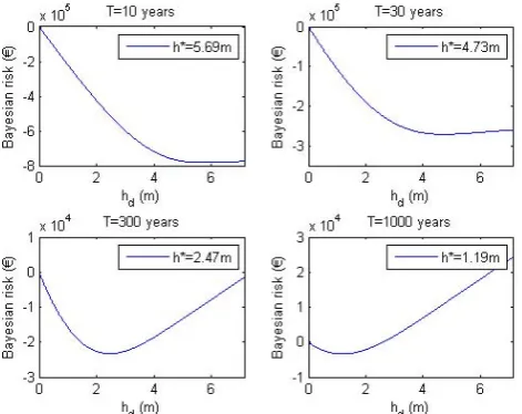
in-creases with the hazard magnitude. And for a given hazard magnitude, the optimal dam height decreases and drops to zero when the distance between the building and the dam in-creases, which indicates that for a building situated very far away from the dam, the defense structure is not efficient at all from a strictly economic point of view. For instance, Fig. 6 shows that the optimal dam height decreases from 5.69 m to 1.19 m when the return period of the considered abscissa in-creases from 10 to 1000 years (Table 2). The corresponding expected benefit is very high for abscissa corresponding to “small” return periods, e.g., C 782 000 for a building situ-ated at a 10-year return period abscissa, because in this case numerous avalanches that would have destroyed the building without the dam are stopped by the dam before the building (Table 3). But the optimal height is then very poorly defined with a rather constant benefit for 5 m≤hd<7.14 m. On the
Fig. 6. Sensitivity of the Bayesian risk function to the position
of the exposed building. aλ0=31.001,bλ0=28.01,a0ρ=1208.7 and
bρ0=28.01.Co=5530 C .m−1,C1=300 000 C,α=0.1376,ho=1 m
andA=25.
expected benefit is so small (around C 3000 at the optimal dam height) that the principle of a dam construction must be questioned.
Finally, it should be noted that a significant difference be-tween the classical and Bayesian optima exists for all build-ing positions, with alwaysh∗B≥h∗C andb∗B≥b∗C. Moreover, these differences increase with the return period of the build-ing abscissa, for example from 5% to 250% for the optimal height (Table 2) and from 8.7% to more than 1250% for the expected benefit (Table 3) for building abscissas correspond-ing to return periods rangcorrespond-ing from 10 to 1000 years. Tak-ing estimation error into account therefore affects especially the optimal design of a defense structure protecting buildings threatened only by the most extreme events. This result is quite intuitive given that estimation error particularly affects the evaluation of the highest quantiles of the hazard distribu-tion, making extreme runout distances more probable than if perfect knowledge of the hazard is assumed.
4.4.2 Hazard frequency
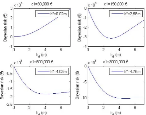
The damage term of the risk function is directly proportional to the mean avalanche frequency. This explains that the higher the mean avalanche frequency, the higher the optimal dam height. Moreover, the expected benefit is nearly propor-tional to the avalanche frequency for small dam heights. For example, the Bayesian optimal height drops to 2.98 m and the corresponding expected benefit is nearly halved if the excee-dence rate drops from 0.9 to 0.45 avalanches.year−1, whereas the optimal dam height increases to 4.03 m and the corre-sponding expected benefit is nearly doubled if the avalanche rate increases from 0.9 to 1.8 avalanches.year−1(Fig. 7).
Fig. 7. Sensitivity of the Bayesian risk function to the an-nual avalanche rate. a0λ=31.001, aρ0=1208.7 and bρ0=28.01.
xb=xstop100, Co=5530 C .m
−1, C
1=300 000 C, α=0.1376,
ho=1 m andA=25.
4.4.3 Cost ratio
The effect of costs on the risk function can be studied by considering the ratio between the construction price and the actualized damage costA×C1
Co . As one would expect, there is a minimal value of the ratio for the optimal height to exist. Figure 8, for instance, indicates that when the ratio is divided by ten by setting the building value to C 30 000 instead of C 300 000, this minimal ratio is nearly attained, so a dam construction is not advisable. Conversely, for very high val-ues of the ratio, the optimal dam height increases only slowly with the ratio because the dam is already high enough to stop nearly all avalanches before the exposed building. For ex-ample, Fig. 8 shows that if the ratio is multiplied by ten, the optimal height is only 0.72 m higher than if the ratio is multi-plied by two. Moreover, for such high values of the ratio, the optimal height becomes poorly defined, with the risk func-tion having a shape very close to what is observed in Fig. 6 for small building abscissas. Between the extreme cases of a very small or a very high cost ratio, the optimal height is well defined.
4.4.4 Parameterα
Fig. 8. Sensitivity of the Bayesian risk function to the
destruc-tion cost. a0λ=31.001, bλ0=28.01, aρ0=1208.7 and b0ρ=28.01.
xb=xstop100,Co=5530 C .m−1,α=0.1376,ho=1 m andA=25.
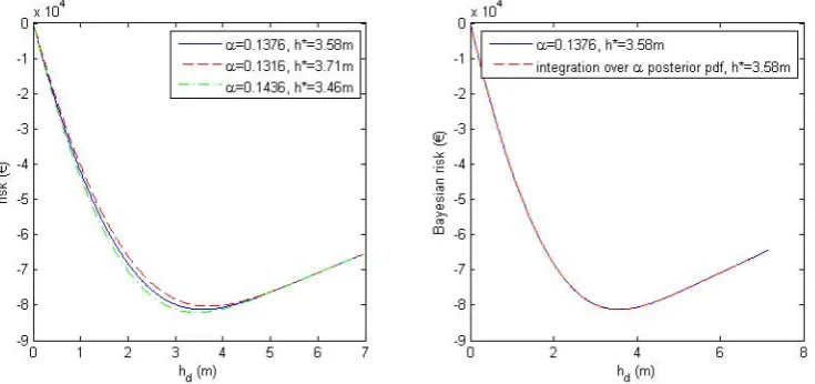
height, with an optimal design of 3.71 m instead of 3.46 m if the more pessimistic value ofαis retained.
Alternatively, it can also be considered thatαis a param-eter of the model and that the true Bayesian risk function has to be obtained by integrating over its posterior distribu-tion. Hypothesizing independence between α and the pa-rameters of the hazard model, the true Bayesian risk func-tion RB0 (hd) is then given by Eq. 24 wherep (α|data)is
the posterior distribution ofα derived from the analysis of the small-scale experiments. The latter one is Gaussian if a conjugate normal-inverse Gamma model is considered for the linear regression (e.g., Gelman et al., 1995). However, it must be integrated numerically. Figure 9 (right) compares RB(hd), andR0B(hd), showing no sensitivity to the
uncer-tainty concerningαfor the case study.
R0B(hd)=Eα[RB(hd)]=
Z
RB(hd)×p (α|data)×dα (24)
5 Discussion
5.1 Hazard variability: POT model versus reality 5.1.1 Topographic dependence
For physical variables such as river discharges, POT mod-els rely on mathematical justifications, with Pickands (1975) proving an asymptotic convergence of any tail of distribution to a POT model where the magnitude follows a generalized Pareto distribution as soon as the threshold is high enough. For snow avalanche runout distances, this theoretical justi-fication does not, however, hold because the distribution of runout distances depends substantially on the slope profile
(Meunier and Ancey, 2004; Eckert et al., 2008a). Neverthe-less, a type of POT model known as the runout ratio model is well known in the avalanche field and it has been used for more than 20 years by avalanche practitioners. In this model, the exceedences of the so-called Beta point corresponding to the beginning of the runout zone are normalized using to-pographic characteristics of the path (to compare data from different paths) and then fitted using extreme value distribu-tions (McClung and Lied 1987; McClung, 2000; McClung, 2001; Keylock 2005). The choice of the threshold is not based on theoretical considerations (Coles, 2001). The key point is that the statistical model is then considered an empir-ical model rather than a true limit distribution. It is applied to very regular paths only, so as to make assumable the as-sumption that the exceedence probability of a given abscissa depends on the normalized distance with the beta point only. This pragmatic point of view is also adopted in this paper. We use a POT model with a threshold fixed by topographic considerations and an imposed exponential tail, which is as-sumed to give a realistic representation of the variability of avalanche runout distances on a regular path. The hypothesis of the independence between runout distances and local con-cavity changes appears in the risk functions obtained, which depend only on the distance between the dam and the build-ing.
5.1.2 Monovariate versus multivariate
Beyond the problem of the topographical dependence, the choice of a POT model for avalanche runout distances can also be severely questioned because it offers only a mono-variate vision of avalanche hazard. For instance, the flow depth that is necessary for the computation of the influence of the dam has to be assumed constant from one avalanche to another, which is not very realistic because a significant cor-relation between runout distances and flow depths may exist for some paths.
Fig. 9. Sensitivity of the Bayesian risk function to theαparameter. α. a0λ =31.001,b0λ=28.01,aρ0=1208.7 andb0ρ=28.01.xb=xstop100,
Co=5530 C .m−1,C1=300 000 C,ho=1 m andA=25.
5.2 Influence of the dam: linear relation for granular media versus reality
Beyond the problem of sensitivity to the value of the param-eterα, the model of the influence of the dam on runout dis-tances used in this paper should also be questioned. It was obtained by an approximated theoretical computation and verified by analyzing small-scale experiments with noncohe-sive rapid granular flows impacting a vertical dam. Its exten-sion to full-scale avalanches overtopping a dam remains an open question even if a partial validation has been recently suggested (Faug et al., 2008). The relevance of the compu-tations proposed to engineering practices is therefore limited to the case of a vertical avalanche dam impacted by rapid noncohesive flows.
In reality, however, different kinds of avalanches are ob-served because of the changing nature of the fluid involved (Ancey, 2006) and only dry dense snow avalanches – which are characterized by densities around 300 kg.m−3, flow paths following the topography, and a low level of cohesion – cor-respond to the experimental case. Moreover, the engineering practice generally considers different geometries of passive defense structures. This preliminary approach therefore de-serves to be further detailed by incorporating the influence of other types of hazards (wet snow avalanches, powder snow avalanches, etc.) on different defense structures (deflective dams, protective mounds, etc.), so as to propose different tools for the various situations that can be encountered in an operational context. Working with a numerical multivariate avalanche model would then be helpful, so as to describe the variability of the relevant quantities.
5.3 Cost quantification
5.3.1 Global economic value versus reality
For a risk computation on a real case study, the elements at risk are not limited to a single building at a fixed position and the number and nature of the exposed buildings, their furni-ture, the number of inhabitants and the fraction of time they live inside, etc., have to be counted and evaluated. This task can be achieved using an interdisciplinary approach (Fuchs et al., 2004; Fuchs and Br¨undl, 2005; Keiler, 2004). A crit-ical point is how to take into account human lives. Mathe-matical convenience is to follow insurance techniques and to give an economic value to a human life. Alternatively, all the computations can be carried out by considering only human lives and expressing the cost function in terms of probabil-ity of being killed, as in the Icelandic legislation for hazard mapping (Arnalds et al., 2004). Since this is not the focus of the paper, this problem was overlooked by considering only a global economic value for a single building situated at a fixed position of the runout zone. Obviously, if several buildings with furniture, cars, etc., are approximatively situated at the same abscissa, the formalism remains identical. This is also true if the choice is made to give an economic value to a human life. If not, however, the cost formulation has to be reconsidered.
5.3.2 Hypothesis for cost modelling
to obtain a more realistic representation of the cost increase with the dam height increase.
The hypothesis of an unbreakable dam could also be re-laxed with an additional term quantifying the mean annual repair cost. However, with a well-designed dam (a very long structural return period such as 300 years), the mean annual reconstruction cost is small with respect to the mean annual damage to the exposed building, so that it can be neglected in a preliminary approximation. Moreover, the repair cost can be simply included in the construction costCowith the
definition of an amortizing period and a computation of its total actualization, as is done in Sect. 2.2 for the damage to the building.
For the damage cost, modelling improvements are much less straightforward. The damage inflected by a snow avalanche to a building is known to depend on impact pres-sure, flow depth, variation of the pressure with time, etc. But the relation between hazard magnitude and damage inten-sity is still unclear (Keylock and Barbolini, 2002; Berthet-Rambaud, 2004). In addition, the impact pressure itself re-mains hard to quantify (Sovilla et al., 2008), so that empirical velocity-dependant damage formulations are generally con-sidered (Jonasson et al., 1999; Barbolini et al., 2004a). Our step function, obviously a very rough approximation, can therefore be justified by the current lack of knowledge. How-ever, this preliminary approach has a direct interpretation in terms of maximal loss (total destruction of the building), and is therefore well suited for the quantification of the maximal expected benefit of the dam construction. Moreover, it can be amended using the more complex damage formulations proposed in the literature and involving other variables such as velocity or pressure. This will be done in association with the multivariate hazard model and the numerical computa-tions of the risk funccomputa-tions mentioned earlier.
6 Conclusion and relevance for practical applications
In this paper, a general Bayesian framework for optimal design of an avalanche dam was proposed, with particular attention given to the problem of handling the uncertainty stemming from the lack of local information from inference to decision. The other major difference with previous risk computations in the avalanche field is the explicit incorpo-ration of a passive defense structure in the modeling frame-work and its optimization with regards to the full variability of the damageable phenomenon. Such an approach can be contested if a specific protection against very frequent or ex-tremely rare events is searched. However, this is a general question in decision theory (Berger, 1985). Moreover, it can be argued that the choice of a defense structure that mini-mizes the mean expected loss instead of the loss associated with a given scenario (e.g. centennial) corresponds to a ratio-nal behaviour for a decision maker facing risk.
Strong simplifying assumptions discussed in details in Section 5 have been introduced. They concern the hazard model, the model for dam influence and the cost quantifica-tion. As a consequence, a rough evaluation of the optimal height and of the expected benefit of the dam construction is obtained. On the other hand, theses assumptions allow ob-taining a simple decisional model that proposes an analytical expression of the Bayesian risk function.
As it is shown with the case study, this decisional model highlights the main effects in this type of engineering exam-ple, for instance the more cautious design value that should be recommended when parameter uncertainty is taken into account and the maximal benefit that can then be expected from the dam construction. Moreover, a sensitivity analy-sis for different factors, e.g. avalanche magnitude, avalanche frequency, cost ratios and dissipation power of the dam, can be performed at very low computational costs. It for example shows the increase of the optimal dam height with the value of the elements at risk. The low effective optimal dam height obtained for a building situated at a centennial abscissa has to be attributed to the chosen economic value of the exposed building.
For a real case study, this decisional model can therefore be used as a first approximation to compute an optimal dam height and to perform a sensitivity analysis at no computa-tional cost. However, it has evident limitations. For instance, it can be used only for very regular paths because runout dis-tance distribution depends upon the slope’s profile. More-over, given that avalanche magnitude is limited to runout distance of dense snow avalanches, it is difficult to propose easy analytical improvements of both dam influence and cost quantification.
Appendix A
List of symbols
A total actualization
a generic notation for avalanche frequency
aρ, bρ/a0ρ, b0ρ a priori/a posteriori parameters of the
Gamma distribution ofρ
aλ, bλ/aλ0, b0λ a priori/a posteriori parameters of the
Gamma distribution ofλ b∗
C, b ∗
B expected classical and Bayesian benefits for the optimal dam height
Co( ) total construction cost
C1( ) total damage cost
data local or experimental data
E mathematical expectation
ho reference flow height (height of the
avalanche impacting the dam)
hd dam height
h∗C classical optimal dam height h∗B Bayesian optimal dam height it annual interest rate of the yeart
I{ } indicator function
l( ) stochastic avalanche model
n number of exceedences
m number of years of avalanche survey p( ) posterior distribution
RB( ) Bayesian risk
RB0( ) Bayesian risk integrated over the distri-bution of theαparameter
RC( ) classical risk
T return period
u( ) linear utility
x abscissa
xb building abscissa
xd dam abscissa
xstopT runout distance corresponding to the return periodT
xstopo reference runout distance without dam xstop(hd) modified runout distance with dam
heighthd
y generic notation for avalanche magnitude
z altitude
α parameter quantifying the influence of the dam
δh∗, δb∗ difference between the classical and Bayesian optimal heights, difference be-tween the classical and Bayesian opti-mal benefits
λ parameter of the Poisson distribution of avalancheoccurrences
π( ) prior distribution
ρ parameter of the exponential distribution of runout distances ∧
θ point estimate for the parameterθ θM generic notation for the parameters of
the magnitude model
θF generic notation for the parameters of
the frequency model
Edited by: F. Guzzetti
Reviewed by: two anonymous referees
References
Amzal, B., Bois, F.,Y., Parent, and E., Robert, C. P.: Bayesian-Optimal Design via Interacting Particle Systems, Journal of the American Statistical Association, 101(474), 773–785, 2006. Arnalds, P., Jonasson, K., and Sigurdson, S. T.: Avalanche
haz-ard zoning in Iceland based on individual risk, Ann. glaciol., 38, 285–290, 2004.
Ancey, C.: Dynamique des avalanches. Presses Polytechniques et Universitaires Romandes, 334 p., 2006.
Ancey, C., Gervasoni, C., and Meunier, M.: Computing extreme avalanches, Cold Reg. Sci. Technol., 39, 161–184, 2004. Ancey, C. and Richard, D.: D´etermination de l’al´ea de r´ef´erence.
Rapport Cemagref /M´et´eo France `a la Direction de la Pr´evention des Pollutions et des Risques, 176 p., 2000.
Barbolini, M., Cappabianca, F., and Savi, S.: Risk assessment in avalanche-prone areas, Ann. glaciol., 38, 115–122, 2004a. Barbolini, M., Cappabianca, F., and Sailer, R.: Empirical estimate
of vulnerability relations for use in snow avalanche risk assess-ment, Atti del convegno Risk Analysis 2004, 533–542, 27–29 Settembre, Rodi, Grecia, edited by: Brebbia, C. A., 2004b. Bardou, E.: R´eglementation en Suisse, in: Dynamique des
avalanches, C. Ancey dir., Presses polytechniques et universi-taires romandes, 334 p., 2006.
Bayes T.: Essay Towards Solving a Problem in the Doctrine of Chances, Philosophical Transactions of the Royal Society of London, 53, 370–418 and 54, 296–325, 1763.
B´elanger, L. and Cassayre, Y.: Projects for past avalanche obser-vation and zoning in France, after 1999 catastrophic avalanches, Proceedings of the International Snow Survey Workshop, 19–24 September 2004, Jackson Hole, Wyoming, 416–422, 2004. Berger, J. O.: Statistical Decision Theory and Bayesian Analysis,
Second edition, Springer-Verlag ed., 617 p., 1985.
Bernardo, J. M., and Smith, A. F. M.: Bayesian theory, Wiley ed., 586 p., 1994.
Bernier, J.: D´ecisions et comportements des d´ecideurs face au risque, Journal des Sciences Hydrologiques, 48(3), 301–316, 2003.
Berger, J. O.: Statistical Decision Theory and Bayesian Analysis, Second edition, Springer-Verlag ed., 617 p., 1985.
Berthet Rambaud, P.: Structures rigides soumises aux avalanches et chutes de blocs: mod´elisation du comportement m´ecanique et caract´erisation de l’interaction ph´enom`ene-ouvrage. Doctorat sciences et g´eographie, sp´ecialit´e: m´ecanique et g´enie-civil. Uni-versit´e Joseph Fourier, Grenoble, 285 p., 2004.
fully developed flows, Ann. glaciol., 38, 30–34, 2004.
Chernouss, P. A. and Fedorenko, Y.: Application of statistical sim-ulation for avalanche risk evaluation, Ann. glaciol., 32, 182–186, 2001.
Clark., J. S.: Why environmental scientists are becoming Bayesians, Ecol. Lett., 8, 2–14, 2005.
Coles, S.: An introduction to statistical modelling of extreme val-ues, Springer ed., 208 p., 2001.
Dent, J. D. and Lang, T. E.: Modelling of snow flow, Journal of Glaciology, 26–94, 131–140, 1980.
Eckert, N., Parent, E., and Richard, D.: Revisiting statistical – to-pographical methods for avalanche predetermination: Bayesian modelling for runout distance predictive distribution, Cold Reg. Sci. Technol., 49, 88–107, 2007.
Eckert, N., Parent, E., Naaim, M., and Richard, D.: Bayesian stochastic modelling for avalanche predetermination: from a general system framework to return period computations, Stoch. Env. Res. Risk. A., 22, 185–206, 2008a.
Eckert, N., Parent, E., Faug, T., and Naaim, M.: Bayesian opti-mal design of an avalanche dam using a multivariate numerical avalanche model, Stoch. Env. Res. Risk A., in press, 2008b. Faug, T., Naaim, M., Bertrand, D., Lachamp, P., and Naaim-Bouvet,
F.: Varying dam height to shorten the run-out of dense avalanche flows: developing a scaling law from laboratory experiments, Surveys in Geophysics, 24(5/6), 555–568, 2003.
Faug, T.: Simulation sur mod`ele r´eduit de l’influence d’un obsta-cle sur un ´ecoulement `a surface libre, Th`ese de doctorat en Sci-ences de la Terre, de l’Univers et de l’Environnement, Universit´e Joseph Fourier, Grenoble, France, 175 p., 2004.
Faug, T., Gauer, P., Lied, K., and Naaim, M.: Overrun length of avalanches overtopping catching dams: Cross-comparison of small-scale laboratory experiments and observa-tions from full-scale avalanches, J. Geophys. Res., 113, F03009, doi:10.1029/2007JF000854, 2008.
Fuchs, S. and Br¨undl, M.: Damage potential and losses resulting from snow avalanches in settlements in the Canton of Grisons, Switzerland, Natural Hazards, 34, 53–69, 2005.
Fuchs, S., Br¨undl, M., and St¨otter, J.: Development of avalanche risk between 1950 and 2000 in the Municipality of Davos, Switzerland, Nat. Hazards Earth Syst. Sci., 4, 263–275, 2004, http://www.nat-hazards-earth-syst-sci.net/4/263/2004/.
Fuchs, S., Keiler, M., Zischg, A., and Br¨undl, M.: The long-term development of avalanche risk in settlements considering the temporal variability of damage potential, Nat. Hazards Earth Syst. Sci., 5, 893–901, 2005,
http://www.nat-hazards-earth-syst-sci.net/5/893/2005/.
Fuchs, S. and McAlpin, M. C.: The net benefit of public expen-ditures on avalanche defence structures in the municipality of Davos, Switzerland, Nat. Hazards Earth Syst. Sci., 5, 319–330, 2005,
http://www.nat-hazards-earth-syst-sci.net/5/319/2005/.
Gauer, P. and Kristensen, K.: Avalanche Studies and Model Vali-dation in Europe, SATSIE; Ryggfonn measurements: Overview and dam interaction, NGI Report 20021048-10, Sognsveien 72, N-0806 Oslo, Norwegian Geotechnical Institute, 2005.
Gelman, A., Carlin, J. B., Stern, H. S., and Rubin, D. B.: Bayesian Data Analysis, Chapman & Hall ed, 526 p., 1995.
Girard, P. and Parent, E.: The deductive phase of statistical anal-ysis via predictive simulations: test, validation and control of a
linear model with autocorrelated errors representing a food pro-cess, Journal of statistical planning and inference, 124, 99–120, 2004.
Grˆet-Regamey, A. and Straub, D.: Spatially explicit avalanche risk assessment linking Bayesian networks to a GIS, Nat. Hazards Earth Syst. Sci., 6, 911–926, 2006,
http://www.nat-hazards-earth-syst-sci.net/6/911/2006/.
Harbitz, C, Issler, D., and Keylock, C. J.: Conclusions from a re-cent survey of avalanche computational models, Proceedings of the anniversary conference 25 years of snow avalanche research, Voss, 12–16 May, Norvegian Geotechnical Institute publication, 203, 128–139, 1998.
Hakonardottir, K. M., Johannesson, T., Tiefenbacher, F., and Kern., M.: A laboratory study of the retarding effect of breaking mounds in 3, 6 and 9 m long chutes, IMO Report 01007, VE-DURSTOFA ISLANDS, 2001.
Jonasson, K., Sigurdson, S. T., and Arnalds, P.: Estimation of Avalanche Risk.Vedurstofu Islands, Reykjavik. VI-R99001-UR01, 44 p., 1999.
Jordaan, I.: Decisions under Uncertainty. Pobabilistic Analysis for Engineering Decisions, Cambridge University Press, 688 p., 2005.
Keiler, M.: Development of the damage potential resulting from avalanche risk in the period 1950–2000, case study Galt¨ur, Nat. Hazards Earth Syst. Sci., 4, 249–256, 2004,
http://www.nat-hazards-earth-syst-sci.net/4/249/2004/.
Keylock, C. J. and Barbolini, M.: Snow avalanche impact pressure – vulnerability relations for use in risk assessment, Can. Geotech. J., 38, 227–238, 2001.
Keylock, C. J., McClung, D., and Magnusson M.: Avalanche risk mapping by simulation, Journal of Glaciology, 45(150), 303– 314, 1999.
Keylock, C.: An alternative form for the statistical distribution of extreme avalanche runout distances, Cold Reg. Sci. Technol., 42, 185–193, 2005.
Krzysztofowicz, R.: Why should a forecaster and a decision maker use Bayes Theorem, Water Resources Research, 19(2), 327–336, 1983.
Krzysztofowicz, R.: The case of probabilistic forecasting in hydrol-ogy, J. Hydrol., 249, 2–9, 2001.
Lied, K., Moe, A., Kristensen, K., et al.: Ryggfonn, Full scale avalanche test site and the effect of the catching dam, Pro-ceedings of the symposium Snow and avalanche test sites, 22– 23 November 2001, Grenoble, France, 2001.
McClung, D. and Lied, K.: Statistical and geometrical definition of snow-avalanche runout, Cold Reg. Sci. Technol., 13, 107–119 1987.
McClung, D.: Extreme avalanche runout in space and time, Can. Geotech. J., 37, 161–170, 2000.
McClung, D.: Extreme avalanche runout: a comparison of empiri-cal models, Can. Geotech. J., 38, 1254–1265, 2001.
Merz, B., Kreibich, H., Thieken, A., and Schmidtke, R.: Estimation uncertainty of direct monetary flood damage to buildings, Nat. Hazards Earth Syst. Sci., 4, 153–163, 2004,
http://www.nat-hazards-earth-syst-sci.net/4/153/2004/.
Meunier, M. and Ancey, C.: Towards a conceptual approach to predetermining high-return-period avalanche run-out distances, Journal of Glaciology, 50(169), 268–278, 2004.
pour l’´etude des avalanches, Cemagref ed., 245 p., 2004. Mougin, P.: Les avalanches en Savoie, Minist`ere de l’Agriculture,
Direction G´en´erale des Eaux et Forˆets, Service des Grandes Forces Hydrauliques, Paris, France, 175–317, 1922.
M¨uller, P.: Simulation-based optimal design, Bayesian Statistics, 6, 459–474, 1999.
Naaim, M., Naaim-Bouvet, F., Faug, T., and Bouchet, A.: Dense snow avalanche modelling: flow, erosion, deposition and obsta-cle effects, Cold Reg. Sci. Technol., 39, 193–204, 2004. Parent, E. and Bernier, J.: Bayesian P.O.T. modelling for historical
data, Journal of Hydrology, 274, 95–108, 2003.
Parent, E. and Bernier, J.: Le raisonnement bay´esien : mod´elisation et inf´erence, Springer ed., 380 p., 2007.
Pickands, J.: Statistical inference using extreme order statistics, Ann. Stat., 3, 11–130, 1975.
Sovilla, B., Schaer, M., Kern, M., and Bartelt, P.: Impact pres-sures and flow regimes in dense snow avalanches observed at the Vall´ee de la Sionne test site, J. Geophys. Res., 113, F01010, doi:10.1029/2006JF000688, 2008.
Salm, B. Burkard, A., and Gubler, H. U.: Berechnung von Fliess-lawinen: eine Anleitung f¨ur Praktiker mit Beispilen, SLF Davos technical report 47, 1990.
Wilhelm, C.: Wirtschaftlichkeit im Lawinenschutz, Methodik und Erhebungen zur Beurteilung von Schutzmassnahmen mit-tels quantitativer Risikoanalyse und ¨okonomischer Bewertung, Mitt.Eidgen¨oss, Inst. Schnee- Lawinenforsch., 54, 309 p., 1997. Wilhelm, C.: Kosten-Wirksamkeit von