A multiple scattering problem

Thesis by A. D. Varvatsis

In Partial Fulfillment of the Requirements

For the Degree of Doctor of Philosophy

California Institute of Technology Pasadena, California

1968

ACKNOWLEDGMENTS

The author is grateful to Professor C. H. Papas for his continued guidance and encouragement during the course of this

work. Special thanks are due to Dr. H. Hodara, Mr. Tom McGill Jr. for many helpful discussions, and Mr. P. Marmarelis for assistance

The present work deals with the problem of the interaction of the electromagnetic radiation with a statistical distribution of non-magnetic dielectric particles immersed in an infinite homogeneous isotropic, non-magnetic medium. The wavelength of the incident radiation can be less, equal or greater than the linear dimension of a particle. The distance between any two particles is several wave-lengths. A single particle in the a.bsence of the others is assumed to scatter like a Rayleigh-Gans particle, i.e. interaction between the volume elements (self-interaction) is neglected~ The interaction of the particles is taken into account (multiple scattering) and conditions are set up for the case of a lossless medium which guarantee that the multiple scattering c0ntribution is more important than the self-interaction one. These conditions relate the wavelength A. and the linear dimensions of a particle a and of the region occupied by the particles D. It is found that fo·r constant A./ a, D is proportional to A. and that J

.6x

I

,

where

.6x

is the difference in the dielectric

susceptibilities between particle and medium, has to lie within a certain range.

The total scattering field is obtained as a series the several terms of which represent the corre1>ponding multiple scattering orders.

their Stokes parameters add.

The second and third order intensity terms are explicitly com-puted. The method used suggests a general approach for computing any order. It is found that in general the first order scattering intensity pattern {or phase function} peaks in the forward direction 9

= O.

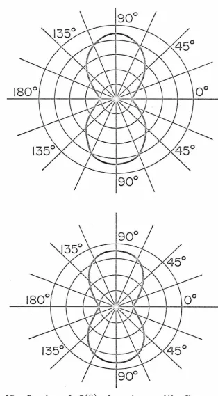
The second order tends to smooth out the pattern giving a maximum in the

a

= 'IT /2 direction and minima in the

a

= 0 ,

a

= 'IT directions. This ceases to be true if ka {where k = 21T/A.) becomes large {> 20). For large ka the forward direction is further enhanced.

Similar features are expected from the higher orders even though the critical value of ka may increase with the order.

The first order polarization of the scattered wave is deter-mined. The ensemble average of the Stokes parameters of the

scattered wave is explicitly computed for the second order. A similar method can be applied for any order. It is found that the polarization of the scattered wave depends on the polarization of the incident wave. If the latter is elliptically polarized then the first order scattered wave

is elliptically polarized' but in the

a

= 'IT/2 direction is linearly polar-ized. If the incident wave is circularly polarized the first order

scattered wave is elliptically polarized except for the directions 9

=

rr/2 {linearly polarized) and 8 = 0, 'IT {circularly polarized). The handedness of the 9

=

0 wave is the same as that of the incident whereas the

elliptically polarized for any 0 no matter what the incident wave is. However, the handedness of the total scattered wave is not altered by the second order. Higher orders have similar effects as the second order.

If the medium is lossy the general approach employed for the

lossless case is still valid. Only the algebra increases in complexity. It is found that the results of the lossless case are insensitive in the first order of k. D where k. = imaginary part of the wave vector

im im

k and D a linear characteristic dimens~on of the region occupied by the particles. Thus moderately extended regions and small losses make (k. D)2

<<

1 and the lossy character of the medium does not

im

alter the results of the lossless case. In general the presence of

PART I II III IV

v

VI

VII

TABLE OF CONTENTS

INTRODUCTION

FORMULATION OF THE PROBLEM 2. 1 Scattering From a ,Single Particle

2. 2 Scattering From a Collection of Particles FIRST ORDER SCATTERING

3. 1 Intensity of the Scattered Wave 3. 2 Polarization of the Scattered Wave SECOND ORDER SCATTERING

4. 1 Intensity of the Scattered Wave 4. 2 Polarization of the Scattered Wave THIRD ORDER SCATTERING

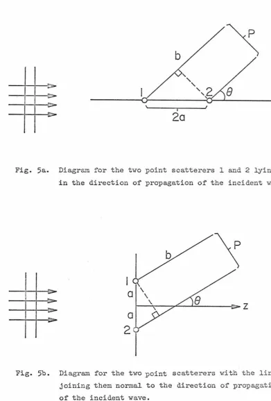
5. 1 Intensity of the Scattered Wave SPECIAL EXAMPLES

6.

1 First Order

6. 1. 1 Two Point Scatterers 6. 1. 2 A Collection of Spheres 6. 1. 3 Needle -like Particles

6. 1. 4 Particles Possessing an Axis of Revolution PAGE 1 5 5 11

29

29

40 44 44 S2 56 56

67

67

69

71

79

85 6. 2 Second Order. General Remarks. Spheres. 90

PART

APPENDICES

P AGE 105 A. The Integral Equation of the Scattering Problem 105

B. The Euler Angles 108

C. Polarization Ellipse. Stokes Parameters. 112

D. Random Sums 115

E. Algebraic and Integral Computations REFERENCES

I . INTRODUCTION

When one computes the scattered wave, due to the illumination

of a collection of particles, ignoring the interaction of the particles

one talks about single scattering. Multiple scattering involves the interaction of the particles.

The first sound attempts to attack the multiple scattering prob-lem are due to Arthur Schuster (1905) who formulated a probprob-lem in

radiative transfer to explain the appearance of absorption and emission

lines in stellar spectra, and to Karl Schwarzschild (1906) who intro-duced and developed the concept of radiative equilibrium in stellar

atmospheres. However, a systematic treatment of the multiple

scatter-ing problem was first given by W. Hartel (9) in 1941. His method is based on determining successive angular intensity distributions for

each successive order of scattering. His theory is applicable to the

case of a medium densely packed with scatterers. This approach has

been recently followed by D. H. Woodward (11) who has assumed that the

scatterers are Mie spheres with a radius large compared to the wave-length. The theory introduced by Hartel, however, does not involve the

polarization of the scattered wave. Such a scalar theory is never

reliable according to Chandrasekhar (8). But Woodward (11) has extended Hartel's theory to include polarization effects.

Another difficulty which also applies to some other theories is the following: One usually starts with the law of single scattering by

talks about the Mie or Rayleigh etc. laws of scattering. Now in a

dense medium every point (small region) is a scatterer. The

inter-action of the scatterers is by far different from the interaction of a

plane wave with a single scatterer. We then understand that when

multiple scattering is taken into account one cannot assume that every

point scatters according to a specified law based on the illumination

of a single scatterer by a plane wave. Therefore, the Hartel theory

cannot use the single scattering theories mentioned above.

In 1945 S. Chandrasekhar (8) developed in a systematic and

mathematically rigorous way the problem of Radiative Transfer. His

equation of transfer is a continuity equation for a 4-dimensional vector

with components the 4 Stokes parameters of the scattered wave. The

radiative transfer theories are best suited to problems such as

scatter-ing by planetary atmospheres, radiative equilibrium of a stellar

atmosphere and other related problems. Like the Hartel theory, the

Radiative Transfer Theories (R. T. T.) assume a medium densely

packed with scatterers. Therefore these theories cannot be based

upon single scattering theories such as Mie's etc. Another frequent

assumption of the R. T .-T. is that the scatterers behave like small

dipoles. If higher moments are taken into account (10) or one

con-siders particles of a shape other than spherical the computations get

pretty complicated.

The theories mentioned above or related ones cannot deal with

the problem of the interaction of a plane wave with a collection of

different from spherical. A rigorous theory for such a situation seems infinitely complicated. If one introduces the element of randomness in the position and orientation of the particles things look brighter. Even so an exact treatment is practically impossible.

The first order scattering or single scattering can be done exactly only when one knows how to find the scattering law for a single particle of a given shape. This is not known in general. A considerable simplification takes place if the single scattering is of the Rayleigh-Gans type, i.e. if the interaction of the volume elements {self-inter-action) is neglected. If one wants to find the effect of the multiple scattering for such particles one must make sure that the multiple scattering contribution is more important than the self-interaction contribution.

Our theory is an approximate one and deals with the following problem. Consider a collection of non-magnetic dielectric particles of any shape immersed in a homogeneous isotropic non-magnetic medium of infinite extent. We will assume that the particles have random position and orientation. The particles are of the Rayleigh-Gans type and are several wavelengths apart. This last assumption is made to simplify the computations.

Consider now a plane wave illuminating the particles. We want to compute the scattered field. The scattered field will be characterized by the four Stokes parameters. The averaging over the random positions

and orientations of the particles will be an ensemble average.

several terms of which represent the corresponding orders of scatter-ing. Thus the first term is a single scattering or first order scatter-ing. The second term is a multiple scattering of the first order or a second order scattering, i.e. the additional current induced within any particle is due to currents inside all other particles induced by the incident field only. The third order involves current due to the second order fields etc.

II. FORMULATION OF THE PROBLEM

2.1. Scattering From a Single Particle

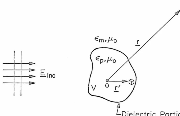
Consider the scattering of a plane wave by a single dielectric

particle (see figure 1). The particle has constitutive parameters E , p

which can be complex, and µ. = µ. = magnetic permeability of vacuum.

p 0

The surrounding medium is infinite, homogeneous, isotropic with

con-stitutive parameters E , complex in general, and µ. = µ. • If we call

m m o

the incident electric field E. and the scattered one E then it can

-inc - s c

·be shown (see Appendix A) that:

Esc(.E) =

w~.6xS!:'(.!i_!

1

)

• E(_E') dV'

c

-v

(2.1.1)

where E(r) =total field at r

=

E. (r)

+ E

(r),

.6x

=

X - X =

- - - -inc - - s c - m p

E - € E - € .

1 1 ik

I

r - r '

I

( m o)

-

( p o )

=

-

(

€ - € ) , I'( r; r r)

= (

u

+

-2

'V

'V

)

e 4

I

- - t

I

Eo Eo Eo m P = - - = k

rr_E-.!

where u

₌

= unit dyadic

=

e e

+

.e e

+ e e

, k

=

wVµ. E •

-~x -y-y -z-z o m

2. 1. 1 can be solved by an iteration method. Thus the first

order approximation is obtained by replacing E(r') by E. (r'): - - i n c

-(2.1. 2)

The second order approximation replaces E(_E ') in ( 2. 1. 1) by

E { r ') = E. ( r ')

+ E[

1] ( r 1 ) :

-p

Em,flo

I

>

>

--

~inc

-~

Loielectric

Particle

Fig. 1. A dielectric particle i l lu.rninated by a plane wave

E.

P

is the observation point.

~

dV"

f

dV'

=

E[ 1](r}

+

E(Z} (r}

- S C - - SC - (2.1.3}

It is now easy to see that in general we must have:

E[n](r}

=

E( 1 } (r}

+

E(Z} (r}

+ ••• +

E(n- 1 } (r}

+

E(n} (r} (2. 1. 4}

- s c - - s c - - s c - - s c - s c

-with

E[O]

=

E. (r}

-sc inc

-• {Srcr

₌

₂;r₃} •••

{Sr

₌

er ₁;r ) • E. (r } dV }

-n- -n -inc -n n

v

v

(2.1.5}

The first order approximation E[i] (r}

=

E(i}(r} is called the Born

- s c - s c

-approximation. From. 2.1. 5 we see that the nth order in the series

believe that for sufficiently small

i

.tix

I the Born approximation is

valid. However, this is not true as the following analysis shows:

Let's compare E(i} to E(Z}, i.e. let's estimate the absolute value - SC - S C

of the fields. We are usually interested in the far zone values (see

Appendix A}

=

w2. .tix

S

I'(r;r'} • E. (r'} dV'

2. _ - - inc

-c

-v

2.

s

ikr - ike • r 1

W e r

E l.k. r

1

::::: -

.tix

(u - e e ) - - e - - • e - dV'

2.

=

- r - r 4irr - o

c

v

"k "k I

w2.

= -

-.tix

_2. 1 r

s

-1 e • r "k

1

e - r - i • r

(e Xe X E ) - - e e -

-- r -- r --o 4irr dV' (2.. 1. 6)

c

_v

dV" dV'

S

e iklE'-..!:"1 _E i·k·.r"

dV" dV' • _,,4-ir'""'l_r....,,-_-r ... "...,.I - o e

-v

S

e ik IE' - ..!: II I

• E

-o

_v

4

Ir' - r" I

1T -

-ik• r II

e - - dV" dV' (2..1.7}

If we assume that k is real then

Is

e

-ik~r·E.'

e -ik·r' - _dV'

I

<

v

S

I

e -ike • r' . - r -

e

1

~·

..!: ,

I

dV'

=

V p

=

volume of dielectric particle. If k is

v

not real then by writing k

=

_{- r} k + ik.

- 1

we get I=

I

S

e-ik~r·.E'ei~·..!:'

dV'

I

v

S

k.e •r' -k.•r'

< e i-r - e - i - dV'. Assuming that E.

-inc travels in the z direction V

s

ki

(~r

-

~z)

• ..!: '

we have I :S e dV'.

v

In the present work we deal with lossy media with k. of the order

l

1 -1

of (1...;.

20)m or less. Therefore in view of the small dimensions of k. (e - e ) • r 1

the particle (< 10 µ) we understand that e 1 - r -z ~ 1 and I

::=

V • Thus

Next we estimate

I

E(2)

j:

- s c

2 2

jE(2)

I

<

(~

jllx

1)

- s c 2

c

l

ikr

I

s -

ike • r '

_e__ e - r - (u + _1_ V''V'')

4rrr

=

k2

v

S

iklr'-r11

I

.

11

• E e - -

e

1

~·

.E.

dV 11 dV' - o 4rr l.E' - ..!: II

I

v

p

(2. 1. 8)

2 2

l

ikr

I

s

s

ik

I

r 1

- r"

I

.

11

<(~It::.

J

)

_e_ lu+-1 V''V'')•E e - -

e1~·r

dV11jdV'

2 X 4irr

=

k2 - o 4irjr1-r11 j

-For estimation purposes we may write \71

,.., _!_ e ' _1· e

k - r • • •

( 2 ) 2 . 2\ ikr

IS

Ir

ikj_!:'-..!:"l

IEsc j< (:2 j.6x I) e4irr 21Eoj

J

e4irl!..'-..!:"I

v

v

e1"k - • E. II dV" dV'

I

To estimate the integral

S

I r•=r" I dV" we choose a spherical

v

-particle of radius a and· we measure ..!:' •..!:" from the center. Then

the integral is the electric potential of a uniform spherical charge

distribution with p = 1 in electrostatic units. evaluated at r' lying

within the sphere. The result is well known:

and

Finally

v

2

~Va ·

p

2 2

I

ikr

I

jE(2) I<

(w

2 l.6x 1) IE Iv a

2

_~

4

-sc - o p irr

c

If we now compare l E ( 1 ) I given by 2. 1 • 8 and

-sc

2. 1. 9 we understand that

(2. 1. 9)

j E(2)

I

given by

- sc .

Condition 2.1.10 further guarantees that

jE~~

j

<<

jE~~-

1

)

j as we

can show, therefore the Born approximation is valid only if 2. 1. 1 O

is satisfied. This condition has been discussed and derived in a

different way by Van de Hulst (2).

2. 2. Scattering From a Collection of Particles

If the scattered electric field by the ith particle (E., µ ) is

l 0

i

called E (r) then the total scattered field is s c

-N

Es c (_!:)

=

l

E~c

(_!:) i=1

where N is the number of particles that do the scattering.

where

If we apply 2. 1.1 for the ith particle we have:

Ei (r)

- s c -

=

w~

c 6x.Sr{r;r.)•E{r.) l = - - 1 - - 1 dV. l

v.

_l

N

E{r.)

=

E. {r.)

+ \

Ej {r.) - -1 -inc -1

L

- s c -1

j=1

(2. 2. 1)

{2. 2. 2)

To be able to write down a series expansion for the total scattered field

as we did in section 2. 1 for a single particle we work as follows:

First we write down the formula for the scattered field by the / h

. 1 h" h. d . "d h .th . 1

part1c e w ic in uces a current lns1 e t e i partlc e. According

to 2. 1. 1 we have:

Ej {r.) -sc - 1

=

w2

2

6x .

S

T{r.;r.)•E'{r.) dV.

J = - 1 -J - -J J

c

v.

J

where

E(r.) = E. (r.) - -J -inc -J

k

E (r.) - s c -J

Next we compute Ek (r.) using 2.1.1 once more. - s c -J

where

k w2

s

E (r.)

= -

₂ .6xk T(r.;rk)• E(rk) dVk - s c -3 c = -J - -

-vk

E(!k)

=

Einc(,Ek)

+

l

E!c(!k)

1

1

Again we use 2.1.1 to compute Esc(,Ek) etc.

(2. 2. 4)

We are now in a position to obtain the series expansion for

N

E (r)

= \

E i (r). The first order term is obtained from 2. 2. 2 if -sc -

6

s c

-i=!

we replace E(r.) by E. (r.), i.e. - - i -inc - i

and

E[i]i

=

w

2

.6X.

S

I'(r;r.)• E. (r.) dV.

=

E(i)i(r) - s c _c 2 i - - - i -inc - i _- i s c

-v.

i

w

2

2 .6x.

S

I'(r;r.)• E. (r.) dV. c i = - - i -inc - i i

v.

_i

The next approximation replaces E(r.) by E. (r.)

+

- - i -inc -i

(2. 2. 5)

N

\ E(i)j(r.),

Li

- S C -J

j=1

E[2] i(r} = w

2 2

6x

.

s

T(r;r.}o E. (r.) dV. - s c - c i = - - 1 -1nc-1 i

v.

l

2 2 ~

+

(w

2) 6X.

S

T(r; r.)• {· \ 6X. Sr(r. ;r.) • E. (r .)dV .}dv. c l = - -1

!.;

.

J = -1 -J -inc -J J l

v

.

J·=1

v.

l J

(2. 2. 6) N

E~~

(E) =

l

E~~]

i(E)

i= 1

N

l

[2]°

To get the third order order E(r.) is replaced by E. (r.)

+

E 1(r.)

- - 1 -inc - 1 - s c - 1

j= 1

i.e.

• E. _{-inc -}(rk) dVk ] dV.} dV. _J

l

= E(i)i(r)

+

E(2)i(r)

+

E(3)i(r) - s c - - s c - . s c

-(2. 2. 7)

N

E[ 3] (r)

= )

E[ 3] \r) - s c - L.J sc

It is clear now how to obtain the

N

th

n order.

replace E(r.} by E. {r.)

+ \

E[n-1] j(r.}. i.e.

- - 1 -inc - 1

6

-sc - 1

j=1

We have to

2 N

+~

eix.S

r(r;r.>·

I

E[n.-1Jj(r.) dV. 2 l - - - 1 - s c - 1 l

c - .

v.

J=1

l

=

E(1)i(r)

+

E( 2)i(r)

+ •••

-sc - -sc -

+

-sc E(n-1)i(r) -

+

- s c -E(n)i(r)

The several terms in the series expansion have a simple

physical explanation which goes as follows:

(2. 2. 8)

The first order scattered field E(1) (r) is due to currents induced by

S C

-the incident field only, i.e. ignoring interaction of -the volume elements

within a particle or of the particles.

The second order scattered field E(2)(r) is due to currents induced by

sc

-the first order scattered field E{1)(r), i.e. a first order interaction

S C

-between volume elements and particles is taken into account.

There-fore, the field E(2) (r) is due to a multiple scattering. sc

-The third order E(3) {r) is due to currents induced by the second order

S C

-E(2)(r) etc. All the terms E{n){r) with. n

>

1 are multiple scattering

-sc - sc

-terms.

Next the following observation should be made.

for example (see 2. 2. 6)

Consider E(2)i

E{2)i

_{= (}

2. 2 N .

w

2) 6 X .

S T(

r; r.) • { \ 6 X .

ST(

r.; r.) • E. ( r.) d V. } d V. - s c _c 1

= -

- 1 ,{...; J

=

- 1 -J -inc -J J i

v.

J=i

v.

l J

=

(w~)

2

{6x.)

2

Sr(r;r.)·ST{r.;r!)•E.

(r!)

dV~

dV. c l = - - 1 = - 1 - 1 -inc - 1 i i

v.

v.

l l

+ (

w~

·

)

2

{6x

.)sT{r;r.)· { \ 6x .

s

I'(r.;r.)

c i

= -

- 1

L

J

=

-1 -J

v.

j=f:i

v.

l J

• E. {r.) dV. } dV.

-inc -J J i {2. 2. 9)

The first term involves the interaction of the volume elements of the

ith particle which would exist even if all the other particles were

absent, whereas the second term describes an interaction between the

ith particle and all the others.

If we recall the results of section 2. 1 we recognize that the

first term is just E{2){r) in 2o 1. 3o This is a self-field because it

S C

-involves interaction within the particle itself. As we shall later see

the second term in 2. 2. 9 will depend on the density of the particles

whereas the first does not. It is not obvious a priori which term is

the most important. Of course they are both of order {6X) 2 if the

x.

's are comparable but this is not the whole story as we saw in

1

section 2. 1. In the present work we will neglect self fields; therefore,

we should find out under what conditions the self-field terms are

negligible compared to terms due to the interaction of the particleso

from interactions within the particles but depending on the presence

of the other particles whereas the first term in 2. 2. 9 does not. Such

terms exist in the higher order terms. Consider for example E(3)(r).

s c

-If we assume for simplicity that N

=

2 we can write 2. 2. 7 as:

• E. (r") dV" ldv' } dV

-me 1 1 J 1 1

(2.2.10}

The first term in 2·. 2.10 would exist even in the absence of particle

second term depends on the presence of particle no. 2. Thus

w~

t:ix₂ \ !::'<.E.i;.E.₂)·Einc(!.₂) dV₂ is the first order scattered field due

c

j

-v2

to particle no. 2. This field induces a current within no. 1. The current produces a field which in turn induces a current within no. 1 again. This last interaction is a self-interaction depending on the presence of no. 2. The third term is not of similar nature. Thus

2 ,...

W I

z

t:ix _{1 \ .!:'<.E. 2;.E.1)·Einc<.E.1 ) dV 1 is a first order field due to no.} 1.

c j

-v1

inducing a current within no. 2. This current produces a field which causes a current within no. 1. There is no self-interaction even though no. 1 affects itself through no. 2. The fourth term includes such an interaction, i.e. the field produced by no. 2 induces a current within no. 2 which in turn produces a field acting on no. 1.

We thus see that E{3)

=

E(3) 1

+

E(3) 2 consists of 2 X 2 X 2

=

8 -sc -sc -sc

terms with only two terms without self-interaction. For any N the

terms without self-interaction are N(N - 1)(N - 1), i.e.

l

a i l bij

l

cjk i j:Fi k:Fj whereas the self-interaction terms are N3 - N(N - 1) (N - 1)

=

N3 - N(N2 - 2N

+

1) = 2N2 - N

For N

>

3

Without: With:

N3 - 2N2

+

N = N out 2N2 - N

=

N

w

N t

>

N • Thus as N gets high, whereas the volume

OU W

largest self-interaction term, i.e. E(2) in 2. 1. 3 smaller than any -sc

arbitrary order term E(n) in 2. 2. 8 if we exclude self-interaction -sc

terms. This seems adequate for a theory which neglects self-interaction but it is not. To see this recall the series expansion 2. 1. 4 for the scattered field by a single particle in the absence of the others. If we want the intensity pattern of the scattered field we have to compute the far zone Poynting vector

Thus

S

=

S _r-r e

S ,..,

j

E 12 =

j

E( 1)

+

E(2)

+ • • •

j

2

r -sc -sc -sc

The scattering is not incoherent, i.e.

The terms have been arranged in orde:i,- of magnitude.

(2. 2.11)

Now if we consider the collection of the particles and neglect the self-interaction terms we can show (see Appendix D) that

<

s

r >,..,<

IE

-sc 12>=<

l

-sc E(1)

+

-sc E(2)

+

•

• •

12)

(2.2.12)

randomness in the position and orientation of the particles.

Therefore what we want is to make sure that any term in 2. 2. 12 is larger than ZN Re E(1) • E(Z) >'.c. The multiplication by N is due to

- s c -sc

the assumption of randomness which make the intensities from the several particles add.

We thus have to find the conditions under which

(IE~~l

2

_>1

.

>>2NRe(E~~·E~~*).

c2.2.13)

collection single

of particles particle

We have already estimated

IE~~)

I

and j

E~~

j for the scattering by a single particle (see 2. 1. 8 and 2. 1.

9}.

Thus we can write

2NRe /E( 1 }.E( 2}).

~SC - S C . l singe particle

(2. 2. 14) if loss es are neglected. Notice that due to interference the left-hand side is usually much smaller than the right-hand side.

As we will show later in this work we get the following result for the average jE(n} j 2 if losses are neglected:

- s c

= I

E

I

2 ( w 2

j

.6 X

I)

2n ( - 1 ) 2 N ( N .)n-1

(_Q_

.)n- 1

F~

-1

o c2 47Tr V

32 7T2

for n':/: 1 (2. 2. 15a}

and

(2 .•

z

.

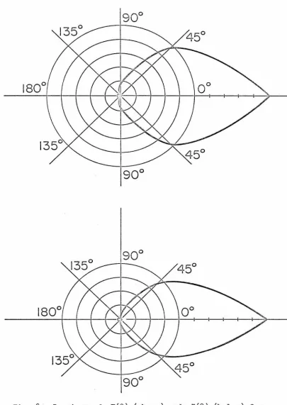
15b)

circularly polarized incident wave. Here V is the volume occupied by the particles. D is a linear dimension of V. F

1 is a function of ka of the order

V~

and K₁• K

2 are given by certain integral ex-pressions which will be later derived. One can see almost by inspec-tion but numerical results for the special case of a collecinspec-tion of

spheres also confirm that K

1,K2 are approximately one order greater than

v

2 if ka is not too large. The maximum value of F(8) is

p

If self-interaction is to be neglected then all multiple scattering terms should be greater than the dominant sel;f-interaction contribution. From 2. 2.14 and 2. 2. 15a we get

On the other hand the series (

I

Esc 12)

=

l (

IE;~)

12) must n

"d . h (

I

Es(nc-1) 12)/(

I

Es(nc)

12)

<<

1. converge rap1 ly, l . e. we must ave

achieve the corresponding conditions we have to notice the following fact. F(8) varies significantly with 8 only when ka is relatively large. In general F(8) is obtained through an averaging procedure and therefore no zeros exist. For the special case of a collection of

To

spheres no averaging takes place and F(e) varies significantly even if ka is not large, i.e. ka::::: 1. On the other hand F(8) has a number

of zeros provided 2 ka

>

4. 5. When F(8)

=

0 then ( /

E~~

J 2) is

.

( I

E(sic) 12) l. s

zero, but the multiple scattering is non-zero, l . e.

should really involve terms with n > 2. One should therefore include the condition

(IE~~

12

>/<

IE~~

12)

<<

1 only when it makes sense.

As we said before in general F(S) has no zeros and unless we

choose ka large F(S) does not vary significantly. For estimation purposes we can write F(S) ;S

V~

and demand

(2.2.17)

as we can easily get from 2. 2. 15a and 2. 2. 1 Sb.

For the ratios with n > 2 we can easily find that 2. 2. 1 7 must

be satisfied.

We can immediately see that 2.2.16 is 11_{hostile" to 2.2.17.} Thus 2. 2. 16 requires high frequencies, high number density whereas

2. 2.17 requires exactly the opposite. The anomaly gets worse as n

increases. Usually however the rapid convergence of the series

( JEsc 12) =

L

(IE~~)

12) guarantees that even a few terms will give

n

an accurate scattering intensity.

We can summarize the· previous discussion as follows. Con-dition 2. 2. 16 requires that

(IE~~)

J 2) >> N 2

Re~~~)E~~>~)

.

single particle whereas 2. 2. 1 7 requires

<

IE(i) 12) >>(E(2) 12) >> •• • >>( - s c - s c IE- s c (n) 12) >>N2Re

(E(1)E(2)>!~)

- s c - s c single . particle

We thus see that ( IE(1) 12) >>N2Re(E(1)E(2)>!'\ .

1 or if we recall - s c - s c - s c

J

sing e

particle

that( jE(i)l 2 ) =NIE( 1 ) 12.

- s c - s c single we get (1E( 1 ) 12)- s c . s.p. >>2Re (E(i)E( 2 )'!<\ . - S C - S C /s.p.

particle

or

I

E(1 )

I

>>

I

E(2)

I

This is, however, condition 2.1. 10. Thus - s c s.p. - s c s.p.

2.1.10 is compatible with the pair 2.2.16 and 2.2.17. As a matter of

fact we can immediately get 2. 1. 10 if we write 2. 2. 16 for n = 2 and combine it with 2. 2. 1 7:

2

w2

l

.6x I

a2

<<

1 • c

To see how 2. 2.16 and 2. 2.17 work we transform them as

follows: The number density

~

can be expressed as 1

3 where

(a +d)

d is an average closest distance between two neighboring particles. This is so because N is approximately equal to N

3 • Here we

(a +d)

should notice that 2. 2. 15 has been derived under the assumption that

the particles are. of such size and so far apart that they only see the

far zone field of any particle. This means that r >> r 1

and kr >> 1

in the expression for I'(_E;_E1

} (see Appendix A).

=

21Tr 21Tr Now k r = - - = - - n

}... }...o m

where n

m is the index of refraction of the medium. Therefore we have the following conditions:

A.o

r >> 2irn m

or

Ao a+ d >>

2'Tl'n m

and a+ d >>a

If we call a+ d = ma then we m ust require that m >> 1 and

Ao A Ao

m>>

2'Tl'n _m a If ~ n > 2rra then m>> 21Tn a implies m>> 1 •

m m

Ao A

i.e. m >> _21Tan suffices. If however

2

<

21Ta m >> 1 does. n

m m

Consider now 2. 2. 16 for n = 2. We will therefore assume that the self-interaction contribution is smaller than the 2nd order multiple

scattering term which is also greater than the 3rd order term in 2. 2.12.

Thus in the present case we will neglect multiple scattering terms

·higher than the second and also self-interaction terms. If we assume the ratio of two successive terms in 2. 2. 12 equal to 10 and the ratio of

the 2nd order multiple scattering intensity to the dominant self-inter

-action term in 2. 2. 11 also equal to 10 then we make a mistake of the

order of 1%. Under the previous assumptions 2.2. 16 and 2. 2.17 give:

2

w

I

A

I

N

~

10 v2 a-2 > 10

- 2

L}x

v

2

c 321T p ·

If we take into account that V p;:::: a3,

~;::::

; ₃ m a transformed into the following:

2

I

I

w D a 1

!::.X c2 3271'2 m3 >

(2. 2.16a)

(2. 2. 17a)

or

3

~<-1_

3 - 100

m

(. D

)-1

3 -1

- - m a

321T2

(2.2.16b)

(2. 2. 17b)

We now understand that if A 2: B and A :S C then C > B, i.e. from

2. 2.16b and 2. 2. 17b:

(2. 2. 18)

i) Assume 21Ta

>

A. /n , i.e. a _{o m}

>

A. _o /21Tn _m • Then we must choose

m

>>

1. If we set m

=

15 then

a :S 9 X 10'""9 D (m

=

15) (2.2.19)

We usually require A.

0 to be in the visible range, i.e.

A.

0

=

4 X

10-5

cm ••• 7 X 10 -5 cm

If we write a

=

nA. /n _{o m} where n is some number greater than 1 /2-rr.

then D must satisfy the following inequality:

n 4 4 7 4 1

D >

U-

(

"9

X 10 cm •••

"9

X 10 cm) (n >

2,,., m

=

15)

m

If for example we choose n/n

=

1/4, i.e. a/A.

=

1/4 then

1 4 7 4

D > {

9

X 1 0 cm • • •

3b

X 10 cm) {m

=

15)

or if n/nm = 5, i.e. a/'11.

0 = 5 then

D :;:::: {

~

X 105 cm • • • 4 X 10 5 cm) {m

=

15)

If we do not specify A

0 we can easily get:

a 6 Ao

n>

₉

10 =p{ka) 18'ITTl

m

{p > 1} {2. 2. 21 a)

Thus if A

0 is constant D increases as ka or a/A increases.

ii) Next asswne 2'lTa

<

A= A /n • Then we should have m>> A /2iran •

o m o m

To comply with case i) we choose m such that ma= 15/k or

m = 15 /ka. We can now easily get

or

7 A

D=p1.7X10 ___2._

{ka)2 nm

Thus if a/A

0 = 1/10 and A0 = 4 X

10-5

with n ~ 1 we get

m

3

D > 1. 7 X 10 cm = 17 m

(2. 2. 21 b)

We observe from 2. 2. 21 b that for A

0 constant D increases as ka or

a/A decreases.

This seems paradoxical since everyone knows that as a/A gets

very small the self-interaction contribution becomes negligible and

therefore 11

the multiple scattering should dominate. 11

However, one

(a/~)

6

whereas the 2nd order multiple scattering like

(a/~)

8, i.e. goes to zero faster. Thus D has to increase to fortify the multiple scattering since N/V is constant for the case a

<

~/2rr. We thus conclude that the minimum D for constant ~ corresponds to ka = 1.

Once we specify a and ~o

= 2rrc/w or better their ratio, as

we show below, we can immediately find the range of

j .6x

I

for which conditions 2. 2.16 and 2. 2. 17 are satisfied. We start from 2. 2.18, i.e.

D 2 3

- - =

p 10 m a 321/

(p > 1)

and conditions 2. 2.16b and 2. 2.17b give:

J.6 x

I

J

.6 x

I

i.e.

2

(

·

~o·)

1 -2 1 3 -1 10-2

>

2rr -p 10 -_{m a} 3- m a

=

-p--_. 2 n

m (ka)2

.

~

2 1 /2 - 2 2

<

(~·)

1 _{10 -2(_1_ ·)} a-3/2m3/2= 10 nm 2rr _p

-:r7Z

_{m a} 3

=172

_p (k ) 2 _a

2 n

m (ka)2

(2. 2. 22)

If ka is large j

.6 x

J has to be small whereas a small ka can make

J.6xJ

of the order unity or larger. Is 2.2.22 the final range of

j.6xJ?

2 How about condition w

2 j

.6

X J a 2

_<<

1 or j

.6

X /

<<

n~/(ka)

2

?

c

2. 2. 1 7a as follows:

we understand that

or

, 2 .)2 N D 2 2

t

~

J.6x

I - -

10

v

\ c2 V 321T2 p

2

w

I

A·

I

2< 1

Z

wX a -100

c

(2. 2. 23)

If we recall that p

>

1 we understand that 2. 2. 22 is the range for

j.6x

j

that satisfies all our conditions.

Next we examine the range of applicability of the theory if

2. 2. 16 with n = 3 holds. Then neglecting self-interaction and higher terms than the third in 2. 2. 12 introduces a mistake of the order of 1

%0

or

less. Remembering that N/V

~

(maf3 • 2. 2. 16 with n = 3 and 2. 2. 17 can be written as

(2. 2. 16c)

1 1/2 D -1/ 2

s

(100) (

321T2)

3/2

m

3/2

a

(2.2.17c)

Again we can easily see that

. ₁ 1/2( D . -1/2 m3/2 _{- l /3} . D . -2/3 m2 (100)

or

3 <

10-4 D

m a - - -₂

3 21T.

(2.2.24)

We can immediately see that the choice of a, A.

0 will be the same as

before {when n = 2 in 2. 2. 16 was chosen) provided D is two orders of magnitude bigger. Therefore, unless very small wavelengths are used, D is too big and the third order is not likely to be practically useful.

The range of

J.6x I

is found easily if we set D/32ir2 =pm3ax104 {p ?.: 1 ) , i. e.

or

2

> 10- 3 nm

J.6 x

I -

-:zy3 - -

₂

p {ka) 2

< 10- 3 nm

l.6

x

I - 772 - -

₂

2 10-3 nm < p2/3 {ka)2

-p {ka)

{p > 1) {2. 2. 25)

Thus if the third order is taken into account D has to get larger and J

.6 x /

has to become smaller than the corresponding quantities in second order.

Do we have to worry about condition

I .6 x

J

<<

n 2 /(ka) 2? No!

2 m

because now 2. 2.16a should read

~

l.6x

J N --22._ 10

v

2 a-2

>

100 and

c2 V 32ir2 p

if it is combined with 2.2.17a we can easily get

J.6xJ

:S 10-3n2 /{ka)2• m

III. FIRST ORDER SCATTERING

3. 1. Intensity of the Scattered Wave

We will assume that the particles in general have different

shapes, random positions and random orientations. They can have

different susceptibilities but of.the same order of magnitude. Later

for the sake of obtaining a simple form for the intensity of the

scat-tered wave we will assume that our particles have the same shape,

dimensions and susceptibilities.

To each particle we attach a triad which will be characterized

by three Eulerian angles (see Appendix B) w. r. t. a fixed system of

orthogonal cartesian coordinates with the z-axis along the wave vector

~ of the incident wave {see figure 2). The Eulerian angles give the

orientation of a particle and will be treated as random variables. We

want to find the far zone scattered field at

.!

characterized by r, 8,cp

w.r.t. the fixed system x,y,z. The expression for the far zone I'

is {see Appendix A)

ikr - ike • r' e r

-; = ( ~ - ~~r) 41Tr e

r

where e

=

-- r r

Therefore we can write for the far zone field given by 2. 2. 5

=

w2

6.x.

_{i e} ikr

s

-ike •r. _{- r - i (}

=

₂ (u e e )

-4- e • E. r.) dV.

- - r - r 1Tr -inc - i i (3.1. 1)

Now E. -inc

-icS

c -

_v.

i

-- E eikz where E h as th e generai · · '"o :i: rm E e

-o -o x

E e Ye i.e. E. is in general elliptically polarized. y -y' -inc

- i cS x

e

x

Einc

_L

y'

Qr

(8,<p)

z'

--z

y

x

A

Fig. 2. x'y'z' is a t r iad attached to the dielectric particle.

xyz is the fixed coordinate frame. e is a uni t

- r

3. 1. 1 can now be rewritten as:

w26x. ikr

s

-ike • r. ikz. 2 1(e Xe - r - r - o XE ) .::__4 irr e - r - 1 e 1 d·V. 1

c

v.

(3. 1 • 2)

l

since e X (e XE ) = e e • E - {e • e )E = {e e - u) • E • Notice that - r - r - o - r - r - o - r - r - o - r - r _ - o

e • E(1 )i{r)

=

0 as it should. To take into account

~he

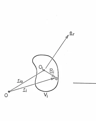
randomness m - r sc

-position of the particles we split r. as follows (figure 3)

- 1

Thus we have

and

r.

=

r.

+

R. -1 -10 -1

r. • e

=

r. • e

+

R .. • e -1 - r -10 - r -1 - r

z.

=

r. • e

=

z.

+

Z.

l - 1 -z LO l

Substituting 3. 1. 4 and 3. 1 • 5 into 3. 1. 2 we get

E (1 )i(r)

=

- s c

-w26x. ikr -ike • r. ikz.

l {e Xe XE ) - 4 e e - r -1oe 10

---=2- - r - r - o irr c

- r - 1 l

S

-ike •R. ikZ.

X e e dVi

v.

l

{3.1. 3)

(3.1.4)

(3.1. 5)

{3.1. 6)

We will temporarily drop the index i. Now we want to evaluate e • R

- r

-and e • R = Z in terms of the Eulerian angles a 1(31 y the polar angles

z

-El ,<p and the coordinates characterizing the shape of the body. If we

0

Fig. 3.

er

- - - J C >

The splitting of r. c r. + R . •

~ ~o ~

r.

'4..0 characterizes the random position of a dielectric particle, whereas

izes the random orientation.

R.

racter-with 0. the center of the ith particle we can view the x'y'z 1 _system

l

as one obtained from xyz by an appropriate rotation, i.e.

-1 I R

1. = (M ) .. R. _{lJ J} (i, j

=

1 , 2, 3; repeated indices are

summed)

where i,j are indices signifying the cartesian components of

R=R.e. =R!e!,

i-1 J.-l

-1

and M is the inverse rotation matrix given by:

cos -y cos (3 - cos a sin (3 s in y - s in )' cos

f3 -

cos a sin

f3

cos y s in a - s in

f3

M-1

=

cos-ysin(3+cosacos(3sin)' -sin)'sin(3+cosacos(3cosy -sinacos(3

and

Now

sinasin-y sinacosy

We now write:

-1 I e • R = (e ).R.'= (e ).(M ) .. x. - r - - r l l - r l lJ J

e • R

=

Z

=

x₃ z

--1 I

=

(M )

3_{J J} .x.

(e )

=

(e )

=

sin ~ sin

e

- r y - r 2

(e ) = (e ) = cos

e

- r z - r 3

cos Ct

I

2 ikr

E ( 1) ( r)

= -

wz

6

x

.

(

e Xe XE ) ! : _ _

4 exp ( - ike • r.

+

ikz. ) - s c - i - r - r - o 1Tr - r - 1 0 lO

. c l

S[

exp '-ik(e )n(8,<pXM-1)n (a.,f3.,-y.)x1 \ - r .x. .x.n l i l n

v.

l

To simplify 3. 1. 7 we define

K.(a .•

!3 .•

-y.;e ,'/>) l l l l

dx' dx'

2 3

(3. 1. 7)

(3. 1. 8)

The time-average radiated power per unit solid angle is given by:

I_ dP

_{- an}

= _r 2 1

_z:

_{Re (E X H • ~r)}

*

In the far zone of a localized source we have:

therefore

2

=

11.

IE I

e

V

µ.o - - r

/Ji

dP 2 1 2

I

= -

=

r - Re

I

E

I

If we substitute 3. 1. 7 into 3. 1.

9

we get

XI\

w₂

2

6x.exp{-ike ·r. +ikz. )K.{a.,13.,"Y.;e,cp}l 2

L

l - r - 1 0 10 l l l l

. c

{3.1.10}

l

To make the computation of 3.1.10 easy to handle we assume that all the particles have the same shape, same size, and same susceptibility. Then we have:

K.{a.

,!3 .•

"Y.;9,<p)

=

K{a. ,13. •"Y·;9,<p}

l l l l l l l

i.e. we drop the index i from K because the functional form will be the same for any particle if all have the same shape and size.

Next we write k

=

k + ik. to take into account the losses of - r l m

the medium. If we now call -k e • r. + k z. = <p., 3.1.10 becomes r-r - 1 0 r 10 l

X

I \'

e i<p i exp /k. { e - e ) • r. ) K {a. ,

l3. ,

"Y.;

e ,

<p) /

2

L

\'.

l m - r - z - 1 0 l l l {3.1.11}

i

We will no·w treat <p. as a random variable {due to randomness

l

( l \

_L

eicpiexp fk.

_\

(e - e }• r . . ) K{a. ,13. ,-y.;0,cp} /

2)

im - r -z - 1 0 1 1 1

i

= N Vi

S

exp { 2k. { e - e ) • a) d V

\ im-r -z

-v

1 s21T

s

2ir

s

1T 2 .

X

-2 jK{a,13,-y;0,cp)j sinadadl3d-y

Sir -y=O 13=0 a=O

{3. 1. 12)

where a is the radius vector from the origin to any point, N the

number of particles and V the volume occupied by the particles.

To estimate the importance of the losses we evaluate

J=

..!..

S

exp

/k.

(e -e )•

~)

dV for an orthogonal parallelopiped

V \'. im-r -z

-v

L ,L ,L •

x y z

L L L

2

_y_

2

1

S

2 2k. e x

s

2 2k. e y

s

2 2k. {e -1)z

J _{= v L e} im rx d _{x L e} im ry d Y L e im rz

_ 2

_

_y_

_ 2

2 2 2

1 1

= -V

3 sinh {k. L e )sinh (k. L e )

k. e e { e _ _1} im x rx im y ry

im rx ry rz

X s inh [ k. L { e - 1 } ]

im z rz

dz

{3.1.13)

Notite that for

e

=0, i.e. forward scattering, J = 1. If we expand

3 x

sinh x = x

+ TI +

we can easily show that 3. 1. 13 gives:

J

=

1

+

O(Lk. ) 2

im (3.1. 14)

Thus J is independent of the loss es, if (k. L) 2

<<

1.

im

1 -1

20 m , therefore a example k. for water can be as low as

im

For

region V with L < 2 m will make (k. L) 2 ::= 1

%

im and J

=

1 with an

error of 1

%.

However, our theory does not allow L to get so sviall

-5 ifthe wavelength is inthe visible range. Thus if A.

0 = (4X10 •••

7X 10-5) cm and n

=

1. 33 then the min L is obtained for ka

=

1, m

i.e. (see 2. 2. 21a)

A.

0

min L

=

₁₈ rrn

m

5.3 m ••• 9.3m

If for example min L

=

5. 3 m then (k. L)2

=

7% and we make an im

error larger than the accuracy of the problem if losses are neglected.

The use of smaller wavelengths can reduce L, also k. = k. (A.) and

im im

then losses can be neglected. If the medium is not too lossy, i.e.

1 -1

kim ;S

100 m then we require L

,2:

10 m and losses can be neg-lected for visible wavelengths and ka of the order unity ~or larger.

We have not worried about the effect of losses on the integral

over a,

l3,

-y for the following reason. If we do the integration we will find a function of

e,

cp and ka. Now k. a will in general be much

im

smaller than unity since a is about the same order as the wavelength.

For example if the medium is water kim::::: 1

-+

~O

m-1 and for the largest k. , k. a ..., 10-7 if A. is in the visible range, whereas

i m i m

k a..., 1. If losses are taken into account we can easily see that they r

tend to reduce the forward scattering.

(3. 1. 13)

where

F(9)

=

~S

2

'1TS

2

'1T

s'IT

IK(a,(3,)';9,cp)l2sina da d(3 d)' (3.1.14)

8'1T -y=O {3=0 a=O

We have written F(9) and not F(9, cp) because the averaging procedure

will eliminate the cp dependence no matter what the shape of the

particles is, provided there are no losses.

Next we compute l!:rX!:rX E

0 1

2

for an elliptically polarized

incident wave. We have

- e Xe XE = component of E perpendicular to e

- r - r - o - o - r

-io

-io

Now E

=

E e

- o x

x

e

-x

+

E y e Ye -y We know that

Thus

and

e

.

e =

-

sin cp e

.

e = cos cp

-x

-cp -y -cp

e

.

!:e = c.os e cos cp e

.

!:e = cos e sin cp

-x

~y

-io

_x

-io

-e X e XE = (- E e sin cp

+

E · e

- r - r -o x y

-io

-io

Y coscp}e

-cp

+

(E cos 9 cos cpe x

+

E e y cos 9 sin cp}!:e

-io -io

=

I -

E e x s in <p

+

E e Y cos <p j2

x

y

-io -io ₂

+

I

E c 0 s e c 0 s <p e x + E c 0 s e s in <p e y

I

x

y

-i{o -o )

=

I -

E e x Y sin <p + E cos <p

I

2

x

y

-i(o -o)

+ cos2ejE e x Y cos<p+E sin<pj2

x

y

= (E cos<p-E cos(o -5 )sin<p)2+cos29(E sin<p+E cos(o -o )cos<p)2

y x x y y x x y

Two special cases are of interest

-io i) E. linearly p.olarized E.

=

E e xe

-inc -inc o -x

-io ii) E. circularly polarized E.

= E

1

e x(e ± ie ).

-inc -inc o -x -y

The plus corresponds to a right-handed and the minus to a left-handed wave.

i) (3.1.16)

The scattered power per unit solid angle is then

(1) 2 2 2 2 2

(I )

a:

NE~(

w

2

Jt:.xi)

(sin <p +cos 9 cos <p)F{8) c

and the intensity pattern of the scattered wave is

1"1")

I

_{~r ~r}

x

x

_{_}E 12 E'2

I

±iir/2 .

+

J 2

0

=

0 e s1n <p cos <p

2 1₂

= (

1 +cos 8)E

0

I.P. ex: {1

+

cos28)F(8)

(3.1.18)

Notice, the intensity pattern is independent of

cp

as i t should be since

the incident wave is circularly polarized,therefore the time average

radiated power per unit solid angle cannot depend on <p. This would

not be true if the collection of the particles exhibited a cp-dependence

on the average.

3. 2. Polarization of the Scattered Wave

Recall equation 3. 1. 7 for the first order total scattered field:

E(l)(r) s c

-'\"' 6 X . exp ( - ike • r. +ikz . ) K. (a. ,

13. ,

y. ; 8 , <p)

3. 2. 1 can be rewritten as

(3. 2. 2)

where the meaning of jF(9,<p,r) leig(S,<p,r) is obvious.

The polarization properties of E(i)(r} entirely depend upon

s c

-the vector e Xe XE which is independent of the material medium,

- r - r - o

the shape, size, orientation and susceptibility of the particles. This

will cease to be true for higher order scattered fields.

-io -io

If E has the form: E e xe

+

E e Ye then we saw in

-o x -x y -y

section 3. 1 that

-io -io

-e Xe XE

- r - r - o =(-Ee x xsin<p + E e

y

Y cos<p)e -<p

-io -io

+(E cos9cos<pe x+E e Yeas 8sin<p}~

0

{3.2.3)

x

y

0

It is obvious from 3. 2. 3 that the total scattered wave is elliptically

polarized. However, for

e

= Tr /2 the polarization is linear since

cos

e

=

o.

To determine the polarization ellipse it is necessary to cast

e X e X E into the following form:

- r - r - o

-io -io

9

- e X e

x

E

=

E<pe <p

~cp

+ E

0 e

~a

- r - r _o o (3.2.4)

It is shown in Appendix C how one can draw the polarization

ellipse if E<p,E

9, o<p, 08 are known. The computation of these

E cos 6 = -E cos 6 sin <p

+

E cos 6 cos <p

<p <p x x y y

E s in 6

= -

E s in 6 s in <p

+

E s in 6 cos <p

<p <p x x y y

and

E 2 = E2 . 2 sin <p + E2 cos 2 <p etc.

<p x

y

The cases of interest are:

-io

i) E. linearly polarized, i.e. E. = e x{E e

+

E e )

-inc -inc x-x y-y

-io

ii) E. circularly polarized, E.

=

E' e x{e ± ie )

-inc -inc o -x -y

i) 3. 2. 3 gives:

-io

- e X e X E = e x

{< -

E s in <p

+

E cos <p) e

- r - r -o x y -<p

The scattered wave is obviously linearly polarized.

ii) 3. 2. 3 gives:

-io

E E ' x( . . )

- e X e X

=

e - s in <p ± i cos <p e

- r - r - o o -<p

-io

+cos 9

E~e

x(cos <p ±sin

<p)~

8

-i{

o

w>

I X

=

E

0 e {cos 9 e -

e

± i e ) -<p

The scattered wave is. elliptically polarized with an inclination angle

ljJ

=

O. However, for 9

=

rr/2 is linearly polarized which is true in

e

=

1T (back scattering) the scattered wave is circularly polarized.

Thus if the incident wave is right-handed circularly polarized then

-e Xe XE - r - r - o

r -i(ox-cp)

=

E e (cos

e

e

0

+

i e )

0 - -cp

e

=

o

=

r -i(o +cp) .

E e x . e l7T( ee- . le )

0 - -cp

e

=

1T

If we take into account the correspondence {x,y,z)~(9,cp,r) we understand that the back-scattered wave is circularly polarized but of opposite handedness than the incident wave whereas the forward

scattered wave is circularly polarized and of the same handedness.

If the incident wave is left-handed circularly polarized then we can easily see that the back-scattered wave is again c.p. but of

opposite handedness whereas the forward scattered wave is c. p. and

of the same handedness as the incident wave.

We can easily understand the above results if we recall that the observer who decides about the sense of rotation of the electric

IV. SECOND ORDER SCATTERING

4. 1. Intensity of the Scattered Wave

Equation 2. 2.

6

gives if the self-interaction terms are neglected:

= { w ₂

2 )

2

6 X .

s

I'( r; r .} • { \ 6 X .

s

I'( r.; r.} • E. ( r.) d V. } d V. \ c l y .

= -

- 1

.L.

J

=

- 1 -J -inc -J J 1

1 J#l V.

J

(4. 1. 1)

We have assumed that the interaction between the particles involves far

zone fields only. Therefore, we can use the simplified form for

I'(r.;r.}

= -1-J

I'(r.;r.}

= -1-J

ikr. - ike • r.

1 - r i -J

~ (u- e e } _e _ _ e _ -r.-r. 4irr.

- l l l

(4.1.2)

If

Ei.

for any particle is measured from a common origin, say the center of the volume occupied by the particles, then 4. 1. 2 is a bad

approximation for particles for which r .- e • r . is close to zero.

1 - r i -J

There are, however, two reasons for using 4. 1. 2. a) The majority

of the particles in pairs satisfies 4. 1. 2 to a good degree of accuracy.

b) Any fine details which would result from an accurate form of

I'(r.;r.) will be completely washed out by.the final averaging procedure.

= -i-J

The scattered field E(2}i(r) is a far zone field, therefore

- S C

-r(r;r.} takes the simplified form 4. 1. 2.

=--1

in the following form

-4 ikr

s

-ike • r.

=

w ₆ e ( ) - r -i.

4

Xi 4rrr ~- ~~r • e

c

-v.

l.

ikr. e l.

-ike •r.+ikz.

{l S

- r i -J (u-e e )•E

-- -r.-r. - o 4rrr.

- l. l. l.

j:;Ci

J .6 X· e

J

v.

J

dV. }dV. J l.

(4. 1. 3)

To take account of the randomness in position of the particles we do the same splitting as we did in section 3. 1, i.e.

r.

=

R.

+

r. -i. -i. -i.o

whereupon 4. 1. 3 becomes

r . = R.

+ r.

-J - J -JO

4 ikr - ike • r.

r

= ~.6.x.-e--(u-e e )·e - r -i.oj(u-e 4 i. 4rrr _ - r - r _ -r.

c - - l

v.

l

-ike r. +ikz.

e )

- r . l

. _e ikri -ike • R. _{- r - 1}

{l

·E - - e x.e

J

-rcJo JO - o 4rrr.

l j:;Ci

-ike • R. "kZ

s

e - r i -J / j dVj}

v.

J

(4. 1. 4)

When we do the integration over the volume of the ith particle we can replace e by its average value e • The reason is the

- r . - r .

following. e

- r .

l

l. 10

particle is situated near the origin then any other particle lies at a

distance much greater than a wavelength. On the other hand the linear

dimensions of the particles are of the order of a wavelength, therefore

the change in the direction of e over the volume of the ith particle - r.

l

is really negligible for all the particles but the one situated near the

origin. However the error we make by ignoring the particle near the ikr. origin is really negligible if N is large. Next we will replace e

ikr.

l/r.

l

by e 10 /r. which again is O. K. for all the particles away from the

10

center.

We can now write 4. 1. 4 as follows:

(u-e e )•E

- - r. - r . -o

- 10 lO

e

ikr. lO

4-rrr.

10

{s

exp (-ike • R.) - r - 1

v.

l

{ "\:"'

_{.!.._;}

6x.exp(-ik_{J -r. -JO} e •r. +ikz. _JO )Sexp(-ike _{-r. -J} ·R.+ikZ_J .) dVJ. }

.=/:. 10 V lO

J l j

(4.1. 5)

If we now recall definition 3. 1. 8 and use 4.1. 5 we get for the total

scattered field:

4 ikr

I

=

~ _e _ _ (u - e e )· 6X .{u - e e ) 4 4-rrr - - r - r l _ - r. - r.

c - . - 10 10

l ikr.

10

• E exp(-ike • r. ) e

4 L.(a.

,13

.

,'f.; 9 ,<p) - o - r - 1 0 rrr. l l l l

lO

{l

j

exp ( -ike • r. + ikz. ) K. (a. ,

13.

,

'Y. ; 9. , <p. ) }

where we have defined

L.(a.,13.,y.~8,<p)

=

Sexp(-ike •R.) dV.

l i l l - r - 1 i

v.

i

To make 4. 1. 6 look simpler we define

(4.1.6a)

)~

.cix. exp(-ike ·r. +ikz. )K.(a.,!3.,y.;8. ,<p. )= A

1(8. ,<p.)

L I J - r

1.0 -JO JO J J J J lO lO lO lO j:i"i

Next we drop the index o as redundant and 4. 1. 6 becomes

4 ikr

E(Z)(r)

=

w _e _ _ (u - e e ) - s c - _c r 4lTr

=

- r - r

ikr.

• { \ .6 X. ( u - e e ) • E exp ( - ike • r.) e

1

~ i = -ri-ri - o - r - 1 4lTri l

L.(a.,!3.,y.;8,cp)A

1(8.,cp.)l

l l l l l l J

It is shown in Appendix D that if E = E(i)

+ E(Z)

+ • • •

then -sc -sc - s c

*

<

- s c - s c E ·E•!<)

=

(E(i).E(- s c - s c 1))

+

(E(Z).E(z)•!<) - s c - s c

+ •••

i.e.

(4. 1. 7)

(4.1.8)

The above relations say that the fields of the several orders are "orthogonal" to each other when the appropriate averaging is done.