http://www.sciencepublishinggroup.com/j/mma doi: 10.11648/j.mma.20190403.11
ISSN: 2575-1786 (Print); ISSN: 2575-1794 (Online)
Application of Homotopy Analysis Method for Solving an
SEIRS Epidemic Model
Inyama Simeon Chioma
1, *, Ekeamadi Godsgift Ugonna
1, Uwagboe Osazee Michael
1,
Omame Andrew
1, Mbachu Hope Ifeyinwa
2, Uwakwe Joy Ijeoma
31Department of Mathematics, Federal University of Technology, Owerri, Nigeria 2
Department of Statistics, Imo State University, Owerri, Nigeria 3
Alvan Ikoku College of Education, Owerri, Nigeria
Email address:
*Corresponding author
To cite this article:
Inyama Simeon Chioma, Ekeamadi Godsgift Ugonna, Uwagboe Osazee Michael, Omame Andrew, Mbachu Hope Ifeyinwa, Uwakwe Joy Ijeoma. Application of Homotopy Analysis Method for Solving an SEIRS Epidemic Model. Mathematical Modelling and Applications; Vol. 4, No. 3, 2019, pp. 36-48. doi: 10.11648/j.mma.20190403.11
Received: June 10, 2019; Accepted: July 15, 2019; Published: September 3, 2019
Abstract:
In this paper, we modified the model of [23] and then applied a new semi-analytic technique namely the Homotopy Analysis Method (HAM) in solving the SEIRS Epidemic Mathematical Model. The modified SEIRS model wasfirst formulated and adequately analyzed. We investigated the basic properties of the model by proving the positivity of the solutions and establishing the invariant region. We further obtained the steady states: disease-free equilibrium (DFE) and endemic equilibrium (EE), then we went further to determine the local stability of the DEF and EE using the basic reproduction number which was calculated. We also applied Lyaponuv method to prove the global stability of endemic equilibrium, The HAM was applied to obtain an accurate solution to the model in few iterations. Finally, a numerical solution (simulation) of the model was obtained using MAPLE 15 computation software.Keywords:
SEIRS Model, Homotopy Analysis Method (HAM), Local Stability, Disease-free Equilibrium, Endemic Equilibrium1. Introduction
Mathematical models have been used in comparing, planning, implementing, evaluating and optimizing various detection, prevention, therapy and control programs.
World Health Statistics (2000) shown that some vector borne diseases as Malaria, Dengue and Yellow fever, continue to threaten throughout the public health of many people. Most of the biological problems are inherently nonlinear.
Modeling of natural phenomena in science and engineering mostly leads to nonlinear problems. Solutions of these nonlinear problems are more difficult compared to linear ones, especially through the analytical approach. Therefore, endless efforts are devoted either to find ways to solve them or to decrease the error in the solutions.
At present, there exist few well known analytical
methods, Homotopy Analysis Method (HAM) gives us an acceptable and more accurate analytical result with convenient convergence and stability.
Homotopy Analysis Method and Modified Homotopy Perturbation Methodwaspresentedfor Strongly Nonlinear Oscillator. In his work he compared the analytical result as well as the numerical result obtained by using Homotopy Analysis Method (HAM), Homotopy Perturbation Method (HPM) and Modified Homotopy Perturbation Method (mHPM). In his study he used different examples with strongly nonlinearity to assess in detail and to illustrate the effectiveness and convenience of the methods. Comparing the three methods with attention focused on the accuracy of the results and applicability of the methods. He came to a conclusion that the solution using HAM which is valid in a small region is more accurate than the solution obtained using other two methods, [18].
Analytic technique, namely Homotopy Analysis Method (HAM) was used for solving an SEIR model. In his work HAM introduced a non-zero auxiliary parameter h to construct a two-parameter family of equations (the zeroth-order deformation equation). The result of the theoretical analysis of the HAM in his work shows that it yields more accurate results in little iteration, [15].
A Homotopy Analysis Method was presented for SEIR tuberculosis model. In their paper, they provided a very accurate, non-perturbative, semi-analytical solution to a system of nonlinear first-order differential equations modeling the transmission of tuberculosis (TB) in a homogeneous population. Their analysis which is based on Homotopy Analysis Method (HAM) used Maple 15 Software to carry out their computations, and their result showed the validity and potential of HAM for computing the solution of nonlinear equations, [7].
An SEIR Model of Seasonal Epidemic Diseases using HAM was presented. The model was centered on childhood diseases measles, chickenpox mumps, rubella incorporate seasonal variation in contact rates due to the increased mixing during school terms compared to school holidays. Driven by seasonality the diseases were characterized by annual oscillations with variation contact rate which is a periodic function of time in years. They used HAM to obtain a semi analytic approximate solution of nonlinear simultaneous differential equations. Mathematical was used to carry out their computations. Result established through graphs showed the validity and potential of HAM for amplitude of Variation greater than zero, [17].
Homotopy analysis method (HAM) was applied to solve Non-linear Cauchy problem. They showed by of means HAM, that the solutions of some linear Cauchy problems of parabolic-hyperbolic type are exactly obtained in the form of convergent Taylor series. The HAM contains the auxiliary parameter, h, that provide a convenient way of controlling the convergent region of series solutions. The results reveal that the proposed method is very effective, [5].
Homotopy analysis method was employed in the analysis of one dimensional heat conduction problem with
temperature dependent thermal conductivity. The temperature distribution is obtained in terms of the scale space variable x and as a function of B which is a parameter in the heat conduction equation. It was observed that the parameter B has a strong influence over the rate of heat conduction in the bar. By choosing the convergence parameter, h, in a suitable way, they obtained solutions for the temperature distribution for various values of B. From this temperature distribution other heat transfer quantities can be obtained. It is observed that for some values of B the temperature distribution in the bar is an increasing function of B while for other values of B it is a decreasing function. In their work, they introduced the basic idea of HAM and applied it to find an approximate analytical solution of the nonlinear one-dimensional heat conduction problem with temperature dependent thermal conductivity, [3].
Homotopy analysis method HAM was applied to solve Convection-Diffusion equation. In their work, the homotopy analysis method was used to find series solution of linear convection diffusion (CD) equation. They further explained that convection diffusion equation is a combination of the diffusion and convection (advection) equations and describes physical phenomena where particles, energy or other physical quantities are transferred inside a physical system due to two processes: diffusion and convection. This equation is a parabolic differential equation which describes physical phenomena. In their work they considered the following linear convection diffusion (CD) equation and the homotopy analysis method was applied to solve it, [4].
Hence, in their work they prove the validity and reliability of the homotopy analysis method (HAM) and with examples showed the accuracy and efficiency of the method. Therefore the homotopy analysis method is able to evaluate a satisfactory solution for convection diffusion equation (CD) Equations.
approximate solutions were in suitable agreement with the exact solutions, thus demonstrating the remarkable efficiency of the homotopy analysis method.
Homotopy analysis method was applied for solving integral and Integro-differential equations. The homotopy analysis method was successfully applied to find the solution of integral and integro-differential equations. It is apparently seen that HAM is a very powerful and efficient technique in finding analytical solutions for wide classes of and integral equations. It is worth pointing out that this method presents a rapid convergence for the solutions. They also do not require large computer memory and discretization of the variables x. Their results show that HAM is a powerful mathematical tool for solving linear equations, [22].
Homotopy analysis method was applied for solving nonlinear Cauchy problem of parabolic-hyperbolic type are exactly obtained in the form of convergent Taylor series. The HAM contains the auxiliary parameter h that provides a convenient way of controlling the convergent region of series solutions. Their results revealed that the proposed method is very effective and simple, [5].
A research carried out that deals with mathematical modeling of malaria transmission in North Senatorial Zone of Taraba State, Nigeria. The SIR proposed by Kermack and McKendrick was implemented using data obtained from Essential Programme on Immunisation (EPI) unit, F.M.C., Jalingo, Taraba state, the data was used to analyse the rate of infection of malaria in the zone. From their analysis, they found out that the reproduction ratio is greater than 0, which implies that the force of malaria infection in Taraba North Senatorial Zone is high. It was recommended specific steps for the reduction of malaria in the zone, [15].
A researcher carried out a review study on mathematical models of malaria with emphasis on their relevance for control. They concluded that; Ross-Macdonald model of malaria transmission has had major influence on malaria control, and that one of its main contributions is that endemicity of malaria is most sensitive to changes in mosquito imago survival rate, and hence malaria can be controlled more efficiently with imagicites than with larvicides. It was further opined that Models that describe the immune response and simulate vaccination programs suggest that one of the most important determinants of the outcome of a vaccine campaign is the duration of vaccine efficacy, [11]. Apparently malaria can be controlled only if the duration of efficacy is in the order of a human life-span.
A mathematical model to study the transmission of malariawas developed; the authors showed from the study
that the model has unique disease-free and endemic equilibria in the application of treatment and preventive measures. We analyze the existence and stability of disease-free and endemic malaria equilibria. Key to their study is the definition of a reproductive number R0 which is the number of the new infections caused by one individual in an otherwise fully susceptible population, through the duration of the infectious period. The disease-free equilibrium is locally asymptotically stable, if R0≤1 and that the endemic equilibrium exist provided R0>1. In fact, their study showed clearly that effective treatment offered to about fifty percent of the infected population together with about fifty percent prevention rate is all that is required to eliminate the disease, [1].
A model was developed and in their model they showed that the three states which a human can be in are; susceptible, infectious and recovered. However, in reality the recovered class is not removed or quarantined from the main population, in fact they become part of the susceptible class. In this work, they present a reviewed dynamical model for the malaria parasite/host dynamics on this basis, [10].
Other papers consulted and referenced are [2, 8, 9, 12, 16, 19, 20]
In this paper, we modified the model of [23]and then solve it with HAM. The total population size N(t) is divided into four compartment, a susceptible compartment, labeled S,( in which all the individuals are vulnerable to the disease but are not yet infected with the disease), an exposed compartment, labeled E,( in which all the individuals are already infected with the disease but are not yet infectious, that is, they cannot infect others with the disease), an infected compartment, labeled I (in which all the individuals are infected by the disease and infectious), a recovered compartment, labeled R in which all the individuals are recovered from the disease and we assume that immunity is not permanent and that recovered individuals do revert to the susceptible class), hence joins the susceptible class again, S. Denote the numbers of individuals in the compartments S, E, I, R, and S, at time t as S(t), E(t), I(t), R(t), and S(t) respectively.
2. Model Formulation
2.1. Flow Diagram
We first draw the flow diagram for [22].
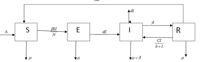
We now present the flow diagram of the modified model.
Figure 2. Flow Diagram of the proposed Model.
2.2. Assumptions of the Model
1.For this model we assume that Immunity is not permanent i.e. Recovered individuals can become susceptible again.
2.We also assume that individuals enter the population by birth or immigration and exist by death or infection.
3.The incidence term is of the standard bilinear mass action this is due to the very large population of infected people and lastly we assume that individuals enter the population by birth or immigration with a constant recruitment as susceptible S and exit by death or by infection.
2.3. Symbols and Parameters
Here we show the description of the symbols and parameter used in formulating the model.
Table 1. Symbols and Description of Model Parameters.
Variables and
Parameters Description
S(t) The number of susceptible individuals at time t E(t) The number of exposed individuals at time t I(t) The number of Infectious individuals at time t R(t) The number of Recovered individuals at time t Λ (t) Recruitment rate
β (t) Effective contact rate
ε (t) The rate at which exposed individuals become infectious γ (t) The rate at which infected individuals recover
ω (t) The rate at which recovered individuals become
Variables and
Parameters Description susceptible µ (t) Natural Death rate N(t) The total population number
2.4. Mathematical Model Formulation
Formulation of the SEIRS mathematical model using the flow diagram above we have:
( )
dS t SI
R S
dt N
β
ω
µ
= Λ + − −
( )
( )
dE t SI
E
dt N
β
µ ε
= − +
( )
( )
dI t CI
E I
dt =
ε
−µ δ γ
+ + −α
+I( )
( )
dR t CI
I R
dt =
γ
+α
+I−µ ω
+( ) ( ) ( ) ( ) ( )
N t =S t +E t +I t +R t
(1)
3. Model Analysis
3.1. Basic Properties of the Model
Note that
( ) ( ) ( ) ( ) ( )
( ) ( ) ( ) ( ) ( ) dN t dS t dE t dI t dR t
N t S t E t I t R t
dt dt dt dt dt
= + + + ⇒ = + + + (2)
( )
( ) ( ) ( )
( )
dN t SI SI CI CI
R S E E I I R
dt N N I I
S E I I R
S E I R I N I
β β
ω µ µ ε ε µ δ γ γ µ ω
α α
µ µ µ δ µ
µ δ µ δ
= Λ + − − + − + + − + + − + + − +
+ +
∴ = Λ − − − − −
= Λ − + + + − = Λ − −
(3)
In the absence of the disease, δ =0, Hence,
( ) ( )
dN t dN t
N N
dt ≥ Λ −
µ
⇒ dt +µ
≥ Λ (4)Using the method of integrating factor we have that the
integrating factor is
dt t
e
∫
µ =eµt t
d N e µ e dtµ
Integrating both sides we have, When
0 0
0, (0)
t N N N c
µ
Λ
= = ⇒ − =
Hence,
0 ( ) 0
t t t
N eµ eµ N N t N e µ
µ µ µ µ −
Λ Λ Λ Λ
• ≥ + − ⇒ ≥ + −
, ( )
As t N t
µ
Λ → ∞ ≥
In the absence of disease, the total population size N(t) converges to the equilibrium
µ
Λ .
From epidemiology consideration, we study our model (1) in the closed feasible region:
(
)
4( ), ( ), ( ), ( ) : ( ) ( ) ( ) ( ) S t E t I t R t S t E t I t R t
µ +
Λ
Ω = ∈ℜ + + + ≥
(5)
3.2. Positivity of Solutions
We show that all the variables in the model equation are non-negative.
Theorem 3.1 (Positivity of Solutions)
Let the initial data for the model (1) be S(0) >0, E(0) > 0, I(0) > 0, R(0) >0. Then the solution set {( ),( ), ( ), ( ) of the model (1) with the positive initial data, will remain positive for all time t > 0.
Proof: Considering the first equation of (2.1) we have
( )
sin
( ) ( )
dS t SI I
R S R S S ce
dt N N
R S S
β β
ω µ ω λ µ λ
ω λ µ λ µ
= Λ + − − = Λ + − − =
= Λ + − + ≥ − +
( ) ( )
( ) ( )
dS t dS t
S dt
dt
λ µ
Sλ µ
∴ ≥ − + ⇒ ≥ − +
( ) ( )
ln ( )S t ≥ − +(
λ µ
)t+c ⇒S t( )≥e− +λ µt c+ e− +λ µt•ec( )
0 0
( ) t, c
S t S e− +λ µ where S e
∴ ≥ =
, ( ) 0
As t→ ∞ S t ≥
Considering the second equation of (2.1) we have,
( )
( ) ( )
dE t SI
E E
dt N
β
µ ε
µ ε
= − + ≥ − +
( )
( ) ln ( ) ( )
dE t
dt E t t c
E ≥ − +µ ε ⇒ ≥ − +µ ε +
( )
0 0
( ) t, c
E t E e− +µ ε where E e
∴ ≥ =
, ( ) 0
As t→ ∞ E t ≥
Following the same way, we can prove that
( ) 0 ( ) 0
I t ≥ and R t ≥
Hence, for t> 0 S(t), E(t), I(t) and R(t) are all non-negative.
3.3. Existence of Steady State of the Model
At steady state
( ) ( ) ( ) ( )
0
dS t dE t dI t dR t
dt = dt = dt = dt = (6)
This implies that
0 SI
R S
N
β
ω µ
Λ + − − =
( ) 0
SI
E N
β − µ ε+ =
( ) CI 0
E I
I
ε µ δ γ α
− + + − =
+
( ) 0
CI
I R
I
γ µ ω
α
+ − + =
+
(7)
Solving (2) we have
* *
0
( )
SI R
R S R S S S
N
β ω
ω µ ω λ µ
λ µ
Λ +
Λ + − − = ⇒Λ + = + ⇒ =
+
* * ( )
( )
SI S
E E N
β µ ε λ
µ ε
= + ⇒ =
+
* *
`( ) 0
( )
CI E C
E I I if
I
ε
ε = µ δ γ+ + +α ⇒ = µ δ γ− α =
+ + +
*
* *
*
( ) 0
( ) ( )
C I
CI I C I
I R R when
I
γ γ
α
γ α µ ω µ ω µ ω α
+
+
+
+ = + ⇒ = = =
* * ( ) R S ω λ µ Λ + = + * * ( ) S E λ µ ε = + * * 0 ( ) E C
I ε if α
µ δ γ − = = + + * * * * 0 ( ) ( ) C I C I I R when γ γ α α µ ω µ ω + + + = = = + + (8)
The disease-free equilibrium is
0 , 0, 0, 0
ξ µΛ
and the endemic equilibrium is
* *
* 0, 0, ,
( ) ( )
E C C I
ε γ
ξ µ δ γ− µ ω+
+ + +
3.4. The Model Basic Reproduction Number
The local stability is established by using the next generation operator method on the system (1).
The Basic Reproduction Number ℜ0 is defined as the expected number of secondary cases produced, in a completely susceptible population, by a typical infective individual [21]. This definition is given for the models that represent spread of infection in a population.
The Basic Reproduction Number ℜ0 is obtained by taking the largest (dominant) eigenvalue or spectral radius of
(
FV 1)
ρ − where 0 0 ( ) ( ) i i i i j j f VF and V
X X ξ ξ ∂ ∂ = = ∂ ∂ i
f = the transmission part which describes the rate of appearance of new infection in theCompartmentiand,
i
V = the transition part which describes the number of ways that individuals can move between Compartmenti,
i i I
V =V−−V+
i
V− = the rate of transfer of individuals out of the compartment i,
I
V+ = the rate of transfer of individuals into the compartment i, by any other means,
0 is the disease free equilibrium,
By linearization approach, the associated matrices at disease free equilibrium are fi and Virespectively. The infected compartments are E and I,
0 i I f N β =
Then we have
0 0 0 i I F N β =
Recall that at DFE,
* S
µ
Λ = , therefore, 0 0 ( 0 0 i N F β µ ξ Λ = Solvingi i I
V =V−−V+
( )
0
( )
i I
E
V CI and V
E I I µ ε ε µ δ γ α −= + += + + + + Hence,
i i I
V =V−−V+is
0
( ) ( ) 0
0 ( )
( ) ( )
i
E E
V CI C
E I I µ ε µ ε ξ ε µ δ γ ε µ δ γ α α + + = − = + + + − + + + + (9) 1 0
( ) 0
1
1
0 1
( ) 0
( )( ) (
1
0 0 0 0
( )( (
C C
N N
N FV
C C
β β
β µ ε
µ µ ε µ δ γ µ µ δ γ
µ ε α α
µ ε µ δ γ α µ δ γ α
−
Λ Λ
Λ
+
+ + + + + + +
= =
+ + + + + + +
(10)
The basic reproduction number is given by (F −1), that is, the highest eigenvalue of FV−1is FV−1−λI =0
1
1
( )( ) ( 0
0
C C
N N
FV I
β λ β
µ µ ε µ δ γ µ µ δ γ
λ α α
λ
−
Λ Λ
−
+ + + + + + +
− = =
−
Hence,
0
( )( C)
N
β
λ λ
µ µ ε µ δ γ α
Λ
− =
+ + + +
1 0 2
( )
and
C N
β
λ λ
µ µ ε µ δ γ α
Λ
⇒ = =
+ + + +
(11)
Therefore, the basic reproduction number is
0
( ) C
N
β µ µ ε µ δ γ
α
Λ ℜ =
+ + + +
(12)
Theorem 3.2: The disease-free steady state is locally asymptotically stable if 0
1
ℜ < and unstable otherwise
.
3.5. Basic Idea of Homotopy Analysis Method
In this section, we apply the Homotopy Analysis Method as proposed by Liao (2004), to solve problem (2.1). Consider the following equation:
N [( )]=0 (13)
where N is a nonlinear operator, t denotes the independent variable. ( ) is an unknown function.
Let 0(t) denote an initial guess of the exact solution ( ), h≠0 an auxiliary parameter, H(t) ≠ 0 an auxiliary function, and L an auxiliary linear operator with the property L [ ( )]= 0 when ( ) = 0. Then using [0,1] as an embedding parameter, we construct such a homotopy.
(1− ) L[∅( , )− 0(t)] − ℎ ( ) [∅( , )] = ̂[∅( , ); 0(t), ( ),ℎ, ] (14) We have the freedom to choose the initial guess 0(t), the auxiliary linear operator L, the non-zero auxiliary parameter h, and the auxiliary function H(t).
Equating the homotopy (5) to zero, that is,
0
( ; ); ( ), ( ), , 0
H⌢Φ t p φ t H t h ρ=
We have the so-called zero order deformation equation
(1− ) L[∅( ; )− 0(t)] − ℎ ( ) [∅( ; )] (15) When = 0, the zero-order deformation equation (15) becomes
∅( ;0) = 0(t) (16)
And when = 1, since h≠0 and H(t) ≠ 0, the zero-order deformation equation (5) becomes
∅( ;1) = (t)
We have the so-called zero order deformation equation
(1− ) L[∅( ; )− 0(t)] − ℎ ( ) [∅( ; )] (17) When = 0, the zero-order deformation equation (17) becomes
∅( ;0) = 0(t) (18)
And when = 1, since h≠0 and H(t) ≠ 0, the zero-order deformation equation (3.8) becomes
∅( ;1) = (t) (19)
Based on (19) and (10), as the embedding parameter increases from 0 to 1 ∅( ; ) varies continuously from the initial approximation 0(t) to the exact solution (t).
Expanding ∅( ; ) in Taylor series with respect to , we have
( ; ) = 0(t) + ∑ ϑm! Σ " ( )# (20)
( ) = !!$& " ∅( ; )/& # " |p=0 (21)
If the auxiliary linear operator, the initial guess, the auxiliary parameter h and the auxiliary function are properly chosen so that
a)The solution ∅( ; ) of the zero-order deformation equation (11) exist for all [0,1]
b)The deformation derivatives * +∅(,;-)
*.+ |p=0 exist for m = 1,2,3,
c)The power series ∅( ; ) = 0(t) +
∑ ϑm(t)∝
! #!converges at =1.
Then, we have under these assumptions the solution series.
∅( ;1) = 0(t) + ∑ ϑm(t)∝
! #! (22)
According to equation (16), the governing equation can be deduced from the zero-order deformation equation (14).
Define the vector
"
= { 0(t), 1(t), 2(t), 1 (t)} (23) Differentiating the zero-order deformation equation (15) mtimes with respect to , then dividing by m! and finally setting 20, we have the so-called mthorder deformation equation.
L[ " ( )3 4 " " 31( )] = hH(t)ℜ" ( " 31( )) (24)
Where
ℜ( " −1( )) = $
!5$
*+6[7(,;8)]
*.+9: (25)
and
0, 1
1 1
m
m
X
m
≤ = >
It should be emphasized that 0(t) for m≥1 is governed by linear equation (20) with the linear boundary conditions that comes from the original problem, which can be solved easily symbolic computation software such as Maple, MATLAB or MATHEMATICA.
3.6. Solution of the SEIR Model byHomotopy Analysis Method (HAM)
In order to explicitly construct approximate non-perturbative solutions of the system described by equations (1), we employ the concept of homotopy analysis method. The advantage of this method is that it provides a direct scheme for solving the problem. To apply the homotopy analysis method, we choose;
S0(t) = Ns, E0(t) = NE, I0(t) = NI and R0(t) = NR.
as initial approximation of S(t), E(t), I(t) and R(t). Let [0,1] be the so-called embedding parameter. The HAM is based on the kind of continuous mappings.
S(t) → ∅1 (t; )
E(t) → ∅2 (t; )
I(t) → ∅3 (t; ) and
R(t) → ∅4 (t; )
such that as the embedding parameter increases from 0 to 1, ∅1 (t; ) varies from the initial approximation to the exact solution. To ensure this, choose such auxiliary linear operators as
Li [; < ( ; # )] = *7=(>;?)
*@ , i= 1,2,3,4,5
With the property
Li [A < ]=0, where A < are integral constants.
We define the nonlinear operators;
1 3
1 1 4
( ; ) ( ; ) ( ; )
[ ( ; )]i i t t t ( '; ) ( , )
N t p t t
t N
φ ρ
βϑ ρ ϑ
ρ
ϕ
= ∂ − Λ + +µφ
ρ ωϑ
−ρ
∂
1 3
2 2
( ; ) ( ; ) ( ; )
[ ( ; )]i i t t t ( ) ( '; )
N t p t
t N
φ ρ
βϑ ρ ϑ
ρ
ϕ
=∂ − +µ ε φ
+ρ
∂
3
3 1 3
3
( ; ) ( , )
[ ( ; )] ( ; ) ( ) ( '; )
( , )
i i
t C t
N t p t t
t t
φ ρ ϑ ρ
ϕ βϑ ρ µ δ γ φ ρ
α ϑ ρ
∂
= − + + + +
∂ +
3
4 3 4 4
3
( ; ) ( , )
[ ( ; )] ( ; ) ( '; ) ( , )
( , )
i i
t C t
N t p t t t
t t
φ ρ ϑ ρ
ϕ γϑ ρ µφ ρ ωϑ ρ
α ϑ ρ
∂
= − + + +
∂ +
Let hi ≠0 and Hi (t) ≠ 0 denotes the so-called auxiliary parameter and auxiliary function respectively. Using the embedding parameter , we construct a family of equations.
(1− ) L [∅1 ( ; ) −B 0 ( )] = ℎ1 1( ) 1[∅1 ( ; )]
(1− ) L [∅2 ( ; ) −C 0 ( )] = ℎ2 2( ) 2[∅2 ( ; )]
(1− ) L [∅3 ( ; ) − 0 ( )] = ℎ3 3( ) 3[∅3( ; )]
(1− ) L [∅4 ( ; ) − 0 ( )] = ℎ4 4( ) 4[∅4( ; )]
Subject to the initial conditions
∅1 (0; ) =B 0 , ∅2 (0; ) =C 0 , ∅3 (0; ) = 0 , ∅4 (0; ) = 0.
of the embedding parameter as follows:
∅1( ; ) = B 0( ) + ∑!D$B!( )#!
∅2( ; ) = C 0( ) + ∑!D$C!( )#!
∅3( ; ) = 0( ) + ∑!D$ !( )#!
∅4( ; ) = 0( ) + ∑!D$ !( )#!
Where, 0 ( ; ) 1 ( ) ! m i m m p t p S t m p ϕ = ∂ = ∂ 2 0 ( ; ) 1 ( ) ! m m m p t p E t m p ϕ = ∂ = ∂ 3 0 ( ; ) 1 ( ) ! m m m p t p I t m p ϕ = ∂ = ∂ 4 0 ( ; ) 1 ( ) ! m m m p t p R t m p
ϕ
= ∂ = ∂L [( ) − 4 " B " −1( )] = ℎ1 1( )ℜ" (B " −1( )
L [( ) − 4 " C " −1( )] = ℎ1 1( )ℜ" (C " −1( ))
L [( ) − 4 " " −1( )] = ℎ1 1( )ℜ" ( " −1( ))
L [( ) − 4 " " −1( )] = ℎ1 1( )ℜ" ( " −1( ))
(0) = 0, (0) = 0, (0) = 0, " (0) = 0.
By the h-curves, it is reasonable to use hi = −1. Using Hi(t) =1 Hence the solution of the " ℎorder deformation equation of the above equations for m≥1 and using h = −1 and H(t) =1 is given by;
1 1 1
m 1 1 1
0
1 1 1
m 1 1
0
1 1
m 1 1 1
( ) ( ) ( ) ( ) ( ) ( ) ( ) ( ) ( ) ( ) ( ) ( ) ( ) ( ) ( ) ( ) ( ) ( ) ( ) ) ( ) t
m m m
m m m m
t
m m m
m m m
m m
m m m m
dS t S t I t
S t S t S t R t dt
dt N
dE t S t I t
E t E t E t dt
dt N
dI t CI t
I t I t E t I t
dt β µ ω β µ ε ε µ δ γ α − − − − − − − − − − − − − − − − = Χ − − Λ + + − = Χ − − + + = Χ − − + + + +
∫
∫
1 0 1 1m 1 1 1 1
1 0 ( ) ( ) ( ) ( ) ( ) ( ) ( ) ( ) ( ) t m t m m
m m m m m
m
dt I t
dR t CI t
R t R t I t R t R t dt
dt γ µ α I t ω
− − − − − − − − + = Χ − − + − + +
∫
∫
3.7. Numerical Solutions
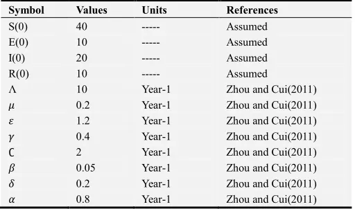
For numerical results, we consider the following values for the parameters involved in the model as presented in Table 2.
Table 2. Parameter values for the series solutions Variables/ Parameters.
Symbol Values Units References S(0) 40 --- Assumed E(0) 10 --- Assumed I(0) 20 --- Assumed R(0) 10 --- Assumed
Λ 10 Year-1 Zhou and Cui(2011)
E 0.2 Year-1 Zhou and Cui(2011)
F 1.2 Year-1 Zhou and Cui(2011)
G 0.4 Year-1 Zhou and Cui(2011)
∁ 2 Year-1 Zhou and Cui(2011)
I 0.05 Year-1 Zhou and Cui(2011)
J 0.2 Year-1 Zhou and Cui(2011)
K 0.8 Year-1 Zhou and Cui(2011)
For high accuracy of results, we use Maple 15 computation software to find the approximate series solution for S(t), E(t),
I(t) and R(t), up to the fifth iteration.
The 1st, 2nd, 3rd, 4th and 5th iterations for S(t), E(t), I(t) and R(t) are calculated and the fifth iteration graphed and presented as below;
First Iteration
1
1
0
( , ) m( ) 40 4.5
m
S x t S t t
=
=
∑
= +1
1
0
( , ) m( ) 10 13.5
m
E x t E t t
=
=
∑
= −1
1
0
( , ) m( ) 20 5.923076923
m
I x t I t t
=
=
∑
= −1
1
0
( , ) m( ) 10 4.923076923
m
R x t R t t
=
=
∑
= +2
2 2
0 2
2 2
0
( , ) ( ) 40 4.5 0.3343750000t
( , ) ( ) 10 13.5 9.404086538t
m m
m m
S x t S t t
E x t E t t
=
=
= = + +
= = − −
∑
∑
2
2 2
0 2
2 2
0
( , ) ( ) 20 5.923076923 5.446005915t
( , ) ( ) 10 4.923076923 2.700147929t
m m
m m
I x t I t t
R x t R t t
=
=
= = − −
= = + −
∑
∑
Third iteration
3
2 3
3
0 3
2 3
3
0 3
2 3
3
0 3
3
0
( , ) ( ) 40 4.5 0.3343750000t -0.2427634215t
( , ) ( ) 10 13.5 9.404086538t -4.438116755t
( , ) ( ) 20 5.923076923 5.446005915t 5.388454330t
( , ) ( ) 10
m m
m m
m m
m m
S x t S t t
E x t E t t
I x t I t t
R x t R t
=
=
=
=
= = + +
= = − −
= = − − +
= = +
∑
∑
∑
∑
2 34.923076923t−2.700147929t -0.4506609387t
The fourth iteratio Fourth iteration
4
2 3 4
4
0 4
2 3 4
4
0 4
2 4
0
( , ) ( ) 40 4.5 0.3343750000t -0.2427634215t 0.05044192265t
, ) ( ) 10 13.5 9.404086538t -4.438116755t 1.582121388t
( , ) ( ) 20 5.923076923 5.446005915t 5.3884
m m
m m
m m
S x t S t t
E x t E t t
I x t I t t
=
=
=
= = + + −
= = − − +
= = − − +
∑
∑
∑
3 44
2 3 4
4
0
54330t -2.538656045t
( , ) m( ) 10 4.923076923 2.700147929t -0.4506609387t 0.7247082028t
m
R x t R t t
=
=
∑
= + − −Fifth iteration
5
2 3 4 5
5
0
( , ) m( ) 40 4.5 0.3343750000t -0.2427634215t 0.05044192265t 0.1067812274t
m
S x t S t t
=
=
∑
= + + − +5
2 3 4 5
5
0
( , ) m( ) 10 13.5 9.404086538t -4.438116755t 1.582121388t -0.4528302558t
m
E x t E t t
=
=
∑
= − − +5
2 3 4 5
5
0
( , ) m( ) 20 5.923076923 5.446005915t 5.388454330t -2.538656045t 0.8347144090t
m
I x t I t t
=
=
∑
= − − + +5
2 3 4 5
5
0
( , ) m( ) 10 4.923076923 2.700147929t -0.4506609387t 0.7247082028t -0.3243836126t
m
R x t R t t
=
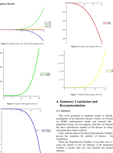
3.8. Graphical Results
Figure 3. Graph of S(t), E(t), I(t) and R(t) against time.
Figure 4. Graph of S(t) against time (t).
Figure 5. Graph of E(t) against time (t).
Figure 6. Graph of I(t) against time (t).
Figure 7. Graph of R(t) against time (t).
4. Summary Conclusion and
Recommendation
4.1. Summary
This work proposed an epidemic model to defend the propagation of an infectious disease. Firstly, we formulated an SEIRS mathematical model and showed that the population classes are non-negative and then we determined the basic reproduction number of the disease by using the next generation matrix method.
Next, with the help of the Basic Reproduction Number, we proved the condition for stability of disease - free - equilibrium.
When the Reproduction Number is less than one, it will cause the disease to die out whereas, if the Reproduction Number is greater than one, this classifies the disease as endemic.
Figure 3.
We went further to adjust the value of the effective contact rate and got a Reproduction Number greater than one, this implies that Disease Free Equilibrium is locally asymptotically Unstable hence this classifies the disease as Endemic. Also this was verified by the Simulation results in Figure 4.
Finally, it is well known that non-linear Ordinary Differential Equations (ODEs) are difficult to solve than linear ODEs, especially by means of analytic methods.
From our numerical solution, we demonstrated the ability of HAM to converge very fast, we saw that the HAM converges in just few iterations. For the accuracy of the method, it has been established by Liao (1992). Hence, we conclude that HAM is a very efficient and accurate method in solving nonlinear mathematical Model.
4.2. Conclusion
After the analysis and simulation study we conclude as follows:
The Model has a Disease Free Equilibrium as
(
* * * *)
0 S E I, , ,R , 0, 0, 0
ξ
µ
Λ
=
The Model also has a Basic Reproduction Number
0
( ) C
N
β µ µ ε µ δ γ
α
Λ ℜ =
+ + + +
Using Table 1 above we got our Reproduction Number 0 = 0.0081 < 1, hence, on average an infected individual produces less than one new infected individual over the cause of his infectious period and the infection cannot grow , hence the Disease Free Equilibrium (D.F.E.), is locally asymptotically Stable and the disease cannot invade the population. This is also shown in Figure 3 above. In the graph, the Susceptible and Recovered goes up hence there is an increase in the Susceptible and Recovered individuals while the graph of Figure 3 the Exposed and infectious goes down hence there is a decrease in the Exposed an Infectious individuals.
Figure 4 above is gotten by changing the effective contact rate I from 0.05 to 7 while all other parameters are left unchanged, hence we got our Reproduction Number 0 = 1.13636 >1 , hence, on average an infected individual produces more than one new infected individual over the cause of his infectious period and the infection can grow, hence, the Disease Free Equilibrium (D.F.E.), is locally asymptotically unstable and the disease can invade the population hence the disease is endemic.
We got our Reproduction Number 0 = 0.0081 < 1, hence this means that on average an infected individual produces less than one new infected individual over the cause of his infectious period and the infection cannot grow , hence the Disease Free Equilibrium (D.F.E.), is locally asymptotically Stable and the disease cannot invade
the population.
This is also shown in the above, in the graph the Susceptible and Recovered goes up hence there is an increase in the Susceptible and Recovered individuals while thegraph of the Exposed and infectious goes down hence there is a decrease in the Exposed an Infectious individuals.
4.3. Recommendation
Globally, diseases have been the major problem to human health, which contributes to the high mortality rate in the world today. Also it thrives in the context of poverty, the costs of seeking accurate diagnosis and treatment can be considerable for low-income household. Infected individuals face substantial cost before diagnosis in that they often consult several public and private providers before and in the process of being diagnosed. Hence in view to these, we therefore recommend that;
The Government, non-governmental organizations and stakeholders should help in creating awareness and preventive measures because prevention is better than cure.
The Government should provide more Hospitals in Nigeria to reduce the high population demand in the exiting hospitals. Infectious Individuals should be properly treated to avoid continuous spread of the disease.
Individuals should shun taking drugs without doctor’s prescription, as this will haveanother side effects.
Finally Homotopy Analysis Method is recommended for further work on non-linear Ordinary differential Equations 50.
References
[1] Avordeh et al (2012) Mathematical Model for the control of malaria- Case study: Chorkor polyclinic, Accra Ghana, Global. Advanced Research journal of Medicine and Medical Sciences, 1 (5) 108-118.
[2] Awrejcewicz, J. et al (1998) Asymptotic Approaches in Nonlinear Dynamics New Trends and Applications; Journal-Springer Series in Synergetics, Publisher Journal-Springer-Verlag berlin Heidelberg ISSN 0172-7389.
[3] Falana, A. and Eighedion, E.E. (2014), Homotopy Analysis Method of one dimensional heat conduction in A Bar with temperature dependent on thermal conductivity. The International Journal of Engineering and Science (IJES) Vol. 3 Issue 5 pages pp-37-46 ISSN (e) : 1813 ISSN (p): 2319-1805.
[4] Fallahzadeh, A. and Shakibi, K. (2015) A method to solve Convection-Diffusion equation based on Homotopy Analysis Method; Journal of Interpolation and Approximation in Scientific Computing. No. (1) 1-8.
[5] Gupta, V. G. and Gupta, S. (2012) Application of Homotopy Analysis Method(HAM) for solving nonlinear Cauchy Problem; Journal-Survey in Mathematics and its Applications, Vol. 7, 105-116 ISSN 1842-6298.
[7] Ibrahim, M. O and Egbetade, S. A. (2013) on the Homotopy Analysis Method for an SEIR Tuberculosis model, American Journal of Applied Mathematics and Statistics Vol1, No pp.71-75.
[8] Jafarian, A. et al (2013) Homotopy Analysis Method for solving coupled Ramani equations. Journal-Rom. J. Phys. 58, 694-705.
[9] Jifeng, C. et al (2015) Homotopy Analysis Method for nonlinear Periodic Oscillating equations with absolute value term Mathematical Problems in Engineering Vol.(7) ID 132651.
[10] Johansson, P. and Leander, J. (2010) Mathematical Modelling of Malaria-Methods for Simulation of Epidemics; A Report from Chalmers University of Technology Gothenbury. [11] Koella, J. C.(1991) On the use of Mathematical Models of
Malaria transmission, Acta Tropical (Elsevier) Vol. 49 pp1-25. [12] Liao, S. J. (2004) Homotopy Analysis Method for nonlinear
Problems; Appl. Math Computer, Vol.174 pp. 449-513. [13] Liao, S. J. (2003) Beyond Perturbation. Introduction to the
Homotopy Analysis Method, Boca Raton Chapman and Hall CRC press.
[14] Lui, G. L. (1997) New research directions in singular Perturbation theory: artificial Parameter method and inverse-perturbation technique conf. of 7th Modern Mathematics and Mechanics, Shanghai, pp.47-53.
[15] Momoh, A. A. et al (2012) Mathematical Modeling of Malaria Transmission in north senatorial zone of Taraba State Nigeria, IOSR Journal ofMathematics, Vol. 3 pp 7-13.
[16] Momoh A. A, Ibrahim M. O. A. Tahir and Ibrahim (2015). Application of Homotopy Analysis Method for Solving SEIR models of Epidemics. Nonlinear Analysis and Differential Equation s Vol. 3, pp 53-68.
[17] Nirmala, P. Subramanian S. P. et al (2015) SEIR Model of Seasonal Epidemic Diseases using HAM. Applications and Applied Mathematics: An International Journal (AAM) vol. 10, Issue pp. 1066-1081 ISSN: 1932-9466.
[18] Srikumar, P. (2013) Assessment of Homotopy Analysis Method and Modified Homotopy perturbation Method for strongly Nonlinear Oscillator, International Journal of nonlinear Science vol. 16 No. 4 pp 291-300 (World Academic Press, England).
[19] Umana, R. A, Omame, A. and Inyama S. C. Global Stability Analysis of the impact of media coverage on the control of infectious diseases. FUTO JNLS 2016 Volume -2, issue -2, Pp.173-194.
[20] Van den Driessche and Watmough (2002) Reproduction numbers and Sub-threshold endemic equilibria for compartmental models of disease transmission; Journal mathematics Biosciences vol. 180 ISSUE 1-2.
[21] Zadeh, K. S. (2010) An integro-patiall differential equations for modellingbiofluids flow in fractured biomaterials, Journal of Theoretical Biology, vol. 273 pp 72-79.
![Figure 1. Flow Diagram of [22].](https://thumb-us.123doks.com/thumbv2/123dok_us/980713.1597666/3.595.138.463.660.738/figure-flow-diagram-of.webp)