University of Pennsylvania
ScholarlyCommons
Publicly Accessible Penn Dissertations
2019
Mendelian Randomization And Single Cell
Deconvolution: Two Problems In Statistics
Genetics
Xuran Wang
University of Pennsylvania, [email protected]
Follow this and additional works at:
https://repository.upenn.edu/edissertations
Part of the
Bioinformatics Commons
,
Genetics Commons
, and the
Statistics and Probability
Commons
Recommended Citation
Wang, Xuran, "Mendelian Randomization And Single Cell Deconvolution: Two Problems In Statistics Genetics" (2019).Publicly Accessible Penn Dissertations. 3325.
Mendelian Randomization And Single Cell Deconvolution: Two
Problems In Statistics Genetics
Abstract
Finding interpretable targets within the genome for diseases is a primary goal of biomedical research. This thesis focuses on developing statistical models and methods for analysis of high throughput genomic and transcriptomic sequencing data with the goal of finding actionable targets of two types, disease-associated genes and disease-implicated cell types.
Traditional genome wide association studies(GWAS) focus on finding the association between genetic variants and diseases. However, GWAS results are often difficult to interpret, and they do not directly lead to an understanding of the true biological mechanism of diseases. Following GWAS findings, we can study the causal effect by Mendelian randomization(MR), which uses segregating genomic loci as instrumental variables to estimate the causal effect of a given exposure to disease outcome. In this thesis, we introduced the concept of ``localizable exposures'', which are exposures that can be localized, or mapped, to a specific region in the genome, such as the expression of a single gene or the methylation of a specific loci. With sequencing technology, allele specific reads are observable for localizable exposures, which allow their quantifications in an allele-specific manner. In the first part of this thesis, we present a new model, ASMR, uses allele-specific information for Mendelian randomization.
This thesis also develops methods for finding cell types implicated in disease through the joint analysis of bulk and single cell RNA sequencing data. Bulk tissue sequencing is often used to probe genes that have tissue-level expression changes between biological cohorts. However, tissue are usually a mixture of multiple distinct cell types and the tissue-level changes are due to shifts of cell type proportions as well as cell type specific expression changes. Single-cell RNA sequencing (scRNA-seq) allows the investigation of the roles of individual cell types during disease initiation and development. We present MuSiC, a method that utilizes cell-type specific gene expression from single-cell RNA sequencing (RNA-seq) data to characterize cell type compositions from bulk RNA-seq data in complex tissues. When applied to pancreatic islet and whole kidney expression data in human, mouse, and rats, MuSiC outperforms existing methods, especially for tissues with closely related cell types. With MuSiC-estimated cell type proportions, we propose a reverse estimation procedure that can detect cell type specific differential expression, allowing for the elucidation of the roles of genes and cell types, as well as their interactions, on disease phenotypes.
Degree Type
Dissertation
Degree Name
Doctor of Philosophy (PhD)
Graduate Group
Applied Mathematics
First Advisor
Keywords
allele, cell type, deconvolution, differential expression, Mendelian randomization, single-cell RNA-sequencng
Subject Categories
MENDELIAN RANDOMIZATION AND SINGLE CELL DECONVOLUTION, TWO
PROBLEMS IN STATISTICS GENETICS
Xuran Wang
A DISSERTATION
in
Applied Mathematics and Computational Science
Presented to the Faculties of the University of Pennsylvania
in
Partial Fulfillment of the Requirements for the
Degree of Doctor of Philosophy
2019
Supervisor of Dissertation
Nancy R. Zhang, Professor of Statistics
Graduate Group Chairperson
Charles L. Epstein, Thomas A. Scott Professor of Mathematics
Dissertation Committee
Nancy R. Zhang, Professor of Statistics
Dylan S. Small, Class of 1965 Wharton Professor of Statistics
MENDELIAN RANDOMIZATION AND SINGLE CELL DECONVOLUTION, TWO
PROBLEMS IN STATISTICS GENETICS
c
COPYRIGHT
2019
Xuran Wang
This work is licensed under the
Creative Commons Attribution
NonCommercial-ShareAlike 3.0
License
To view a copy of this license, visit
ACKNOWLEDGEMENT
First and foremost I want to thank my advisor Nancy Zhang. Without her support and
guidance, I would not have entered the field of statistical genomics. She has taught me,
both consciously and unconsciously, how applied statistics research is done. I appreciate
all her contributions of time, ideas, and funding to make my PhD experience productive
and stimulating. Her enthusiasm for research was contagious and motivational for me, even
through the tough times in the PhD pursuit. The completion of my dissertation would
not have been possible without the support and nurturing of Mingyao Li, who was the
co-advisor for my major research project as well as my committee member. I’m extremely
grateful for the excellent examples Mingyao and Nancy have provided as successful women
researchers and professors. They mentored me on my research, pointed out and helped
strengthen my weaknesses. I’m sure I will benefit from their invaluable words throughout
my academic career. I would also like to extend my deepest gratitude to Dylan Small for
being my co-advisor during my first two year of PhD study and research and my committee
member. He not only taught me statistics, but mentored me with great patience during
my transition period from a student to a beginner researcher. Nancy, Mingyao and Dylan
have demonstrated how good research is done as well as what good researcher (and person)
looks like.
I would like to extend my sincere thanks to Professor Katalin Susztak from Department
of Medicine at University of Pennsylvania as well as Dr.Jihwan Park and Tong Zhou from
Susztak’s group, who kindly shared their data, constructive advice and valuable experiences
during the deconvolution project. I very much appreciate Yan Che, who helped me process
data in the Mendelian randomization project. I must also thank Dr.Charles Epstein, the
graduate chair of Applied Mathematics and Computational Science program, for recruiting
me. Otherwise, I would not have had the opportunity to join Penn and work with those
Special thanks to the members of Nancy’s group, Dr.Jingshu Wang, Chi-Yun Wu, Mo
Huang, Zilu Zhou and Divyansh Agarwal, who have contributed immensely to my personal
and professional time at Penn. The group has been a great source of friendship as well as
good advice and collaboration. I’m grateful for those days and nights we spent together
working in the office, and especially Mo, for helping me edit this thesis. I would also
like to acknowledge friends of Nancy’s group, Dr.Qingyuan Zhao and Professor Jian Ding
for providing encouragements and stimulating motivations. Thanks should also go to my
friends/colleagues at Penn: Lu Wang and Ruoqi Yu, whose professional and emotional
support cannot be overestimated. I’d like to recognize the assistance that I received from
the staff of the mathematics department, statistics department and Wharton computing
group at Penn.
I’m deeply indebted to my parents for being my strongest support and providing endless
and unconditional love. During the tough time of transition from an applied math student
to a beginner researcher of statistical genomics, they never lost faith in me and believed
that I can succeed even though sometimes I did not.
Lastly, I want to thank myself. With my sensitive and sentimental characteristics, I still
made sensible choices. Worn by chronic pains, I never gave up.
Xuran Wang
University of Pennsylvania
ABSTRACT
MENDELIAN RANDOMIZATION AND SINGLE CELL DECONVOLUTION, TWO
PROBLEMS IN STATISTICS GENETICS
Xuran Wang
Nancy R. Zhang
Finding interpretable targets within the genome for diseases is a primary goal of biomedical
research. This thesis focuses on developing statistical models and methods for analysis
of high throughput genomic and transcriptomic sequencing data with the goal of finding
actionable targets of two types, disease-associated genes and disease-implicated cell types.
Traditional genome wide association studies(GWAS) focus on finding the association
be-tween genetic variants and diseases. However, GWAS results are often difficult to interpret,
and they do not directly lead to an understanding of the true biological mechanism of
diseases. Following GWAS findings, we can study the causal effect by Mendelian
random-ization(MR), which uses segregating genomic loci as instrumental variables to estimate the
causal effect of a given exposure to disease outcome. In this thesis, we introduced the
con-cept of “localizable exposures”, which are exposures that can be localized, or mapped, to a
specific region in the genome, such as the expression of a single gene or the methylation of a
specific loci. With sequencing technology, allele specific reads are observable for localizable
exposures, which allow their quantifications in an allele-specific manner. In the first part of
this thesis, we present a new model, ASMR, uses allele-specific information for Mendelian
randomization.
This thesis also develops methods for finding cell types implicated in disease through the
joint analysis of bulk and single cell RNA sequencing data. Bulk tissue sequencing is often
used to probe genes that have tissue-level expression changes between biological cohorts.
changes are due to shifts of cell type proportions as well as cell type specific expression
changes. Single-cell RNA sequencing (scRNA-seq) allows the investigation of the roles of
in-dividual cell types during disease initiation and development. We present MuSiC, a method
that utilizes cell-type specific gene expression from single-cell RNA sequencing (RNA-seq)
data to characterize cell type compositions from bulk RNA-seq data in complex tissues.
When applied to pancreatic islet and whole kidney expression data in human, mouse, and
rats, MuSiC outperforms existing methods, especially for tissues with closely related cell
types. With MuSiC-estimated cell type proportions, we propose a reverse estimation
pro-cedure that can detect cell type specific differential expression, allowing for the elucidation
TABLE OF CONTENTS
ACKNOWLEDGEMENT . . . iii
ABSTRACT . . . v
LIST OF TABLES . . . ix
LIST OF ILLUSTRATIONS . . . xii
PREFACE . . . xiii
CHAPTER 1 : Introduction . . . 1
1.1 Allele specific Mendelian randomization . . . 1
1.2 Cell type contributions to diseases . . . 2
CHAPTER 2 : Allele specific Mendelian randomization . . . 5
2.1 Introduction . . . 5
2.2 Model set up and notations . . . 7
2.3 Estimation of causal effect in allele-specific model . . . 10
2.4 Simulation study . . . 17
2.5 Real data example: Finding downstream targets of lincRNA . . . 20
2.6 Conclusion . . . 27
CHAPTER 3 : Bulk tissue deconvolution with single cell RNA sequencing . . . 28
3.1 Introduction . . . 28
3.2 Methods . . . 29
3.3 Results of deconvolution . . . 41
CHAPTER 4 : Cell type specific differential expression from bulk tissue with single
cell reference . . . 50
4.1 Introduction . . . 50
4.2 Method . . . 52
4.3 Results . . . 59
4.4 Discussion . . . 72
APPENDIX . . . 74
LIST OF TABLES
TABLE 1 : Pancreatic islet datasets . . . 43
TABLE 2 : Mouse/Rat kidney datasets . . . 45
TABLE 3 : Number of differential genes from cell type specific artificial bulk data. . . 67
TABLE 4 : Number of genes that are selected as differentially expressed by MuSiC-DE of cell-type level and by DESeq2 of tissue level. . . 71
TABLE 5 : Linear regression to examine the relation between estimated cell type proportions (Segerstolpe et al. (2016) as reference) and HbA1c levels 76 TABLE 6 : Linear regression to examine the relation between estimated cell type proportions (Baron et al. (2016) as reference) and HbA1c levels . . 77
TABLE 7 : Evaluation of deconvolution methods when there are missing cell types in the single-cell reference . . . 83
TABLE 8 : Starting points for convergence analysis . . . 86
TABLE 9 : Summary of cell types of Park et al. single cell dataset . . . 90
TABLE 10 : Renal tubule segment names. Abbreviations and full names. . . 90
TABLE 11 : List of top 100 high weighted genes from the pancreatic islet analysis 91 TABLE 12 : List of top 100 high weighted genes from the mouse kidney, step 1 of tree-based recursive deconvolution . . . 92
LIST OF ILLUSTRATIONS
FIGURE 1 : Diagram of allele specific Mendelian randomization model . . . . 8
FIGURE 2 : Simulation results when changing instrument strength by the mean
of dosage . . . 20
FIGURE 3 : Simulation results when changing instrument strength by the
vari-ance of dosage . . . 21
FIGURE 4 : Estimated log(|µw|/σu) and log(σw/σu) from first stage likelihood 23
FIGURE 5 : Scatter plot ofXi1 vs. Xi2−Xi1 . . . 24
FIGURE 6 : Scatter plot with histograms of the z-values from ASMR and 2SLS 26
FIGURE 7 : Overview of MuSiC framework . . . 30
FIGURE 8 : Pancreatic islet cell type composition in healthy and T2D human
samples . . . 42
FIGURE 9 : Cell type composition in kidney of mouse CKD models and rat. . 46
FIGURE 10 : Boxplot of estimated cell type proportions for 100 repetitions of
Fadista et al. (2014) dataset . . . 61
FIGURE 11 : Null distribution validation with CPM and log-transformed CPM 62
FIGURE 12 : Scatter plot of true cell type proportions versus estimated cell type
proportions from MuSiC over 100 repetitions . . . 65
FIGURE 13 : Smooth scatter plot of mean and empirical variance of z-values with
selected DE genes. . . 66
FIGURE 14 : Smooth scatter plots of z-values from true proportions and average
z-values from estimated proportions . . . 69
FIGURE 15 : Violin plot of p-values from DESeq2 for alpha and beta cells . . . 70
FIGURE 17 : Simulation results when changing instrument strength by changing
the mean ofW,µw. . . 74
FIGURE 18 : Simulation results when changing instrument strength by changing
the variance ofW,σw. . . 74
FIGURE 19 : Estimated cell type proportions of the pancreatic islet bulk
RNA-seq data in Fadista et al. with single cell reference from Baron et
al. . . 78
FIGURE 20 : Exploratory analysis of single-cell RNA-seq data from Segerstolpe
et al. (2016) single-cell RNA-seq data . . . 79
FIGURE 21 : Heatmaps of true and estimated cell type proportions of artificial
bulk data constructed using single-cell RNA-seq data from Xin
et al. (2016). . . 81
FIGURE 22 : Heatmaps of true and estimated cell type proportions with missing
cell types in single-cell reference. . . 82
FIGURE 23 : Benchmark evaluation of robustness of MuSiC . . . 85
FIGURE 24 : Convergence of MuSiC with different starting points . . . 86
FIGURE 25 : Benchmark evaluation using mouse kidney single-cell RNA-seq data
from Park et al. . . 87
FIGURE 26 : Estimated cell type proportions and correlation of the estimated
cell type proportions of Lee et al. (2015) dataset . . . 88
FIGURE 27 : Estimated cell type proportions of the 13 cell types in tree real bulk
RNA-seq datasets . . . 89
FIGURE 28 : QQ plots of genes with best fit of uniform distribution or worst fit
of uniform distribution. . . 95
FIGURE 29 : QQ plots of DE genes in alpha cells selected by DESeq 2, but not
selected by MuSiC-DE. . . 96
FIGURE 30 : QQ plots of DE genes in beta cells selected by DESeq 2, but not
FIGURE 31 : QQ plots of DE genes in delta cells selected by DESeq 2, but not
selected by MuSiC-DE. . . 97
FIGURE 32 : QQ plots of DE genes in gamma cells selected by DESeq 2, but not
selected by MuSiC-DE. . . 97
PREFACE
This dissertation is submitted for the degree of Doctor of Philosophy at the University
of Pennsylvania. The research described herein was conducted under the supervision of
Professor Nancy R. Zhang and Professor Dylan S. Small in the Statistics Department,
Professor Mingyao Li in the Biostatistics and Epidemiology Department, between May
2015 and April 2019.
This work is to the best of my knowledge original, except where acknowledgements and
references are made to previous work. Neither this, nor any substantially similar dissertation
has been or is being submitted for any other degree, diploma or other qualification at any
other university.
Part of this work has been presented in the following publication:
X. Wang, J. Park, K. Susztak, N. R. Zhang, and M. Li. Bulk tissue cell type deconvolution
CHAPTER 1 : Introduction
A central goal in biomedical research is to study the genome and find genes and other
biological features that are responsible for diseases. Here we refer to such features on which
downstream experiments can be performed to interpret, validate, quantify, and isolate their
functional effects as actionable targets. In this thesis, we developed statistical models and
computational methods for finding actionable targets using genetic and genomic data. The
targets that we consider include the RNA expression of specific gene and the representation
of specific cell types in tissue.
1.1. Allele specific Mendelian randomization
In genetics, Genome-wide association studies (GWAS) have been the stable of research
for the last twenty years, since the sequencing of human genome allowed for the mapping
to genes. The goal of GWAS is to find associations between genetic variants, such as
single-nucleotide polymorphisms (SNPs), and observable traits such as diseases. The first
successful GWAS published in 2002, found the association between LTA and myocardial
infarction (Ozaki et al., 2002). Up until now, we have mapped over a hundred thousand
genetic variants to various diseases, for exampleDRD2 to schizophrenia,PADI4 andIL6R
to rheumatoid arthritis, and more (Visscher et al., 2017). Mapping diseases to genes and
performing downstream analysis allow us to find treatments to diseases with gene
knock-outs, gene editing and developing drugs.
The goal of GWAS is to find genes that are causally implicated in diseases by mapping
diseases onto genetic variants. However, association between genetic variants and diseases
is not enough to establish causal relationships or to explain the underlying biological
mech-anism. From the central dogma of biology, RNA is the intermediate molecule that leverages
the effect of genetic variants to disease phenotypes. This motivates the study of expression
quantitative traits loci (eQTL), defined as genomic loci that explain all or a fraction of
loci and their characterization as eQTLs allow us to quantify the causal effect of gene on
disease phenotypes. The use of inherited genetic variation to study the causal effect of an
exposure on a trait is called Mendelian randomization (MR). In this thesis, we consider
the use of localizable exposures, which we define as exposures that can be localized to a
specific region in the genome. For example, we can think of gene expression or epigenetic
modification as an “exposure” in the terminology of epidemiologists, and since they can
be directly mapping to a genome location, they are localizable exposures. With
sequenc-ing techniques, allele specific reads at heterozygous loci are observable, which allow the
allele-specific quantifications of localizable exposures. We developed a method, ASMR,
that incorporates the allele-specific information in a Mendelian randomization framework
to estimate the causal effect of localizable exposure using maximum likelihood. A
compar-ison of precision between two-stage-least-square (2SLS), a conventional estimation method
for MR, and ASMR is presented with different strength of instrumental variables and
con-founder effects. We also illustrate how to find downstream targets of lncRNA using ASMR.
This work is described in Chapter 2.
1.2. Cell type contributions to diseases
Unlike genetics, which focuses on segregating genetic variants and their affected genes,
ge-nomics is a relatively newer field that involves the whole genome and its quantitative
behav-iors. The technological evolution in whole genome RNA and DNA sequencing have allowed
for genomic studies. A common type of analysis useful in genomics is differential expression
analysis (Costa-Silva et al., 2017), which takes gene expression data to detects quantitative
changes in expression levels between groups of samples such as between disease cohorts.
Es-sentially, for each gene, statistical tests have been developed to decide whether an observed
difference in expression between two cohorts is greater than the expected difference due to
random variation. Large-scaled bulk tissue RNA and DNA sequencing datasets, such as
Genotype-Tissue Expression (GTEx) Project (Carithers et al., 2015), have been generated,
reflects an average over all cells within the tissue, masking the contribution of individual
cell types. It was difficult to sequence at the single cell level before 2009, because it was
hard to isolate individual cells, and because the abundance of RNA in a single cell is too
little to sequence. Recent advances in the techniques for isolating single cells and for
am-plifying their genetic material make possible the exploration of the transcriptome of single
cells. With the birth of single-cell sequencing, researchers can study the transcriptomic
heterogeneity of a single cell for thousands to millions of cells simultaneously.
“Cell type” is a classification used to distinguish between morphologically or phenotypically
distinct cell forms. Usually complex tissues consist of cells of different cell types; for example
in the human pancreas, there are endocrine cell types and exocrine cell types that jointly
regulate glucose level. Cells of the same type show similar transcriptomic pattern, which
can be captured by single cell RNA-seq data. Annotating cell types based on single-cell
transcription profiles is a challenging problem and can be viewed as high-dimensional
un-supervised clustering with high level of biological and technical noises. Currently, popular
clustering methods include Seurat (Butler et al., 2018), TSCAN (Ji and Ji, 2016) and SC3
(Kiselev et al., 2017) (more in the recent review by Du`o et al. (2018)). After clustering,
the cell types are identified by their marker genes, which are genes that only express in a
specific cell type. Based on cell types assigned in this way, we can study the inter- and
intra-cell-type similarity and heterogeneity from single cell sequencing data and develop
methods to study the role of cell types in diseases.
The observed differential expression in bulk tissue is a combined effect of cell type
com-position shifts and the expression shifts within cell types. Therefore, investigating the
differences between groups of samples at the cell type levels can be framed as two problems,
detecting cell type composition shifts and detecting cell type specific differentially expressed
(DE) genes. Finding cell type specific DE genes is especially challenging because there is
confounding from proportion shifts. One may ask, with the rapid adoption of of single cell
due to cell loss in the dissociation and isolation steps of single cell sequencing, proportions
from single cell data do not reflect the true proportions in bulk tissue. Therefore, we and
others(Avila Cobos et al., 2018) proposed the strategy of first estimating cell type
propor-tions of bulk tissues with single cell expression as reference. Such estimation procedures
are often referred as deconvolution. There are many existing deconvolution methods, such
as CIBERSORT (Newman et al., 2015) and BSEQ-sc (Baron et al., 2016). However, they
only use marker genes for estimation and ignore the cross-subject variations of gene
expres-sion when multi-subject single cell datasets are available. We developed a method, MuSiC,
that takes the advantage of cross-subject variations of all genes in deconvolution without
selecting marker genes. This is discussed in Chapter 3.
Now let’s go back to the question of how to detect cell type specific differential expression
from bulk tissue. Cell type specific differential expression testing starts from estimating cell
type proportions by deconvolution guided with single cell reference. Deconvolution methods
with pre-selected marker genes assume that the expression of marker genes are consistent
across healthy and diseased status, which is not always true. For example, in pancreas
islet,INS is the genes responsible for producing insulin and is a marker gene for beta cells.
During the progress of type 2 diabetes, beta cells go through both loss of mass and lack
of function, where there are less beta cells as well as lower INS expression in beta cells for
diseased subjects. Although the expression of INS is higher in beta cells than other cell
types, deconvolution with only marker genes like INS will mistaken the cell type specific
expression changes for cell type proportion shifts. MuSiC eliminates the bias from marker
genes by including all genes for deconvolution. Controlling the estimated proportion from
MuSiC makes it possible to detect cell type specific DE genes between healthy and diseased
status. We proposed a method for testing cell type specific DE genes by comparing two cell
type models with and without disease indicator with a strategy of repetition partition of
genes in to a set used for deconvolution and a separate set on which DE test is conducted.
CHAPTER 2 : Allele specific Mendelian randomization
2.1. Introduction
A common goal of biomedical research is to elucidate the causal roles of genetic and
epi-genetic factors underlying complex human diseases. Mendelian randomization (MR) is a
method for estimating the causal effect of an intermediate variable on an outcome of
in-terest, in which inherited DNA variation are used as instrumental variables to overcome
the effect of confounding and reverse causation. Mendelian randomization was adopted as
early as 1986, when Katan (2004) used genetic markerApoE as instrument for studying the
causal effect of raised blood cholesterol on risk of cancers. Now it has been widely applied
to epidemiology and integrative genetics models, more in the review paper by Burgess et al.
(2017). For example, to measure the causal effect of alcohol consumption on the risk of
coronary heart disease, the genetic variant ALDH2, which reduces alcohol consumption,
has been used as an instrument (Smith and Ebrahim, 2004). In integrative genetics models,
a large number of transcript abundances are measured with the ultimate aim of
identify-ing causal relationships from a morass of expression quantitative trait loci (eQTL) usidentify-ing
Mendelian randomization. For other examples, see recent review by Burgess and Thompson
(2015).
To date, the “modifiable exposure” examined by Mendelian randomization studies have
encompassed blood pressure, obesity, smoking, alcohol intake etc. Increasingly, with the
ubiquitous adoption of high throughput sequencing technologies, the “exposure” of interest
can now also focus in on the expression of a single gene or the methylation of a specific
loci. We call such exposures localizable exposures, in that they can be localized, or
mapped, to a specific region in the genome. High throughput sequencing has revolutionized
the study of the transcriptome and the epigenome. One important benefit of sequencing
is that it quantifies gene expression or epigenetic modification in an allele-specific manner,
example, in RNA sequencing, this allows us to measure the number of transcript copies of
each allele. This allele-level information has not, to our knowledge, been used in Mendelian
randomization studies. We will develop a method for using such allele-level information and
show that it can substantially boost estimation accuracy. Although this chapter focuses
on gene expression, the methods we propose can be applied to other types of localizable
exposures, such as methylation or splicing.
The measurement of allele-specific information in heterozygous individuals enables us to
compare the difference between expressions of two paired alleles and consider expression
level of different genotypes in a causal inference manner, where the causal effect is the
difference between potential outcomes of the same subject. With the same idea, we use
“dosage” to describe the difference between potential expressions of different alleles at the
same loci, thus dosage measures the causal effect of changing the allele. The causal effect
can not be measured directly because at each loci, at each haplotype, only one of the
two potential outcomes can be observed. Even for heterozygous individuals, where the
expression of both allele can be observed, the expression of each allele is a separate random
variable which may be correlated due to the sharing of common environment, but cannot
be considered to have the same potential outcomes.
The focus on localizable exposues has the additional benefit of allowing us to more easily
satisfy the assumptions of Mendelian Randomization. The use of DNA-level variations
as instrumental variables relies on two basic assumptions: First, the DNA variant must
be stably maintained in our cells and not correlated with lifestyle and environment; this
assumption is reasonable in most cases after proper adjustment for genetic ancestry. Second,
the DNA variant must affect the outcome only through the exposure of interest, and this
assumption is often violated, and very difficult to check due to pleiotropy. However, when
the modifiable exposure is localizable, we can select to use only genetic variants that are
physically close to the exposure on the genome. In genetics terminology, we limit our
trans.
The classical approach for analyzing the causal effect in Mendelian randomization is
two-stage least squares (2SLS). As long as the instrumental variable satisfies the assumptions for
being a valid instrument, 2SLS gives consistent estimates of the causal effect of the exposure
on outcome. In this chapter we propose an alternative method for estimating the causal
effect of a localizable exposure on a quantitative phenotype. This chapter is organized as
follows: In Section 2.2, we introduced the additive linear model and our notation. In Section
2.3, we described the model assumption and estimation procedure. Simulation results are
shown in Section 2.4 to compare the powers of the proposed method to 2SLS. We illustrated
the new framework to an example applicable in finding downstream regulatory targets of
lncRNA in the data from the Geuvadis project (Lappalainen et al., 2013). A summary is
given in Section 2.6. To simplify language, we use interchangeably localizable exposure and
gene expression, since the latter is our primary example.
2.2. Model set up and notations
2.2.1. Model overview
Figure 1 shows the relationship between the key variables of our model. LetTi denote the
total expression level for the gene of interest for individual i, i ∈ {1,2, . . . , n}. Yi is the
observed quantitative outcome for individual iand our goal is to estimate the causal effect of changingTi on the outcome Yi. Assume a simple linear model:
Yi=βTi+Vi (2.1)
in whichβ represents the causal effect andVi the total contribution of unobserved covariates
and measurement errors. One could also extend the model to include possible observed
covariates, but since we would be able to control for these by taking partial regression
residuals, leading us back to (2.1), we keep things simple by ignoring observed covariates
Confounder U Observed Expression X Expression T Confounder V Genotype Z Quantitative phenotype Y W Dosage β causal effect ρ Measuremen t error e (a) Homozygous Confounder U Observed Expression
X1,X2
Expression
T1,T2
Confounder V Genotype Z Quantitative phenotype Y W Dosage β causal effect ρ Measuremen t error
e1,e 2
(b) Heterozygous
the individual observations,T= (T1, . . . , Tn)T and Y= (Y1, . . . , Yn)T.
We assume that within the transcribed region of the gene there is a SNP loci, which we
call the tagging SNP, and that located outside the transcribed region incis to the gene is a
regulatory SNP. We also assume that there are only two alleles for each SNP and that the
phase between these two SNPs is known. In other words, we assume that the haplotypes
are known.
The observed total expression, denoted as Xi, differs from true expression level Ti by
mea-surement error ei. For individuals that are heterozygous at the tagging SNP, we observe
the expressions of its two alleles,
Xi1 = Ti1+ei1
and Xi2 = Ti2+ei2,
(2.2)
as well as the observed total expression Xi =Xi1+Xi2; for homozygous individuals, only
the total expressionXi=Ti+ei can be observed. Let Zi1, Zi2 ∈ {0,1}be the two inherited
alleles at the regulatory SNP for individual i. When both the tagging and the regulatory SNPs are heterozygous, let Zi1 and Zi2 correspond to the allele on the haplotype with
expression Ti1 and Ti2, respectively. We assume the additive model for the effect of the
regulatory SNP on the expression of its linked allele,
Tij =Ui+Wi(j)Zij j= 1,2 (2.3)
in which j ∈ {1,2} indexes the haplotype and Wi(j)Zij is the dosage effect of having the
“1” haplotype on expression levelTij. We assume independentcis regulatory effects, which
2.2.2. Two stage least squares method for estimation β
A standardized regression of Y on X would yield a biased estimate for the causal effectβ. This is due to existence of measurement error and correlation betweenU and V. To attain an unbiased estimate, the most widely used method is two-stage least squares (2SLS), which
will be taken as the baseline for comparisons.
2SLS estimates the causal effect β by first forming a prediction for X based on the in-strument Z, and then regressing Y on XZ. In detail, let X˜ = X−X¯, Y˜ = Y−Y¯ and
˜
Z=Z−Z¯, the projection of Xon Zis
XZ = ¯X+ (Z˜0Z˜)−1Z˜0X˜, (2.4)
and the 2SLS estimate ofβ is
ˆ
β2SLS= (X˜0ZX˜Z)−1X˜0ZY˜. (2.5)
The two-stage least squares estimate is a consistent estimator for β in our model, but ignores the information in the allele-specific measurementsXi1,Xi2 for individuals that are
heterozygous at the tagging SNP.
2.3. Estimation of causal effect in allele-specific model
The model described in Section 2.2.1 is a general model void of distribution assumptions.
Here we add specific assumptions on the distribution ofZ,U,V andW to allows maximum likelihood estimation of the causal parameter β.
2.3.1. Distribution assumptions
Assume genotype Zij follows Bernoulli distribution with minor allele frequency P(Zij =
1) = p ∈ (0,1). Without loss of generality, let Zi1 = 1 and Zi2 = 0 when individual i is
In (2.3), the independence of confounderUi and dosage Wi(j) is assumed. This means that
by changing the regulatory SNP’s genotype Zij, the expression difference is independent
of confounder effects contributing to the expression. This is a critical assumption for the
instrumental variable to be a valid one. This assumption is not expected to always be true
and even worse, it is usually hard to verify. With allele specific model, this assumption can
be partially checked byXi1−Xi2s andXi1s from heterozygous individuals, see Figure 5 for
examples. It is intuitive to consider that in (2.1), Vi, the total contribution of unobserved
covariates and measurement errors on the outcome, is also independent ofWi(j). We assume thatWi(j)is i.i.d. normal with mean µw and varianceσw2, and that the joint distribution of
(Ui, Vi) is i.i.d. bivariate normal with correlation ρ,
Ui
Vi
∼N(
µu
µv
,
σ2u ρσuσv
ρσuσv σv2
).
Measurement error ein (2.2) is independent of the other variables. For each observation, measurement error follows N(0, σe2). That is, instead of observing Tij or Ti, we observe
Xij =Tij+eij and Xi =Ti+ei.
Given the observed distribution assumptions, the distribution for the observed data
{Zi, Xi, Yi} for homozygous and{Zi, Xi1, Xi2, Yi}for heterozygous as follows:
For (Zi1, Zi2) = (0,0), i.e. homozygous individuals for the (0,0) haplotype,
(Yi−βXi, Xi)T ∼N((µv, 2µu)T,Σ1); (2.6)
for heterozygous individuals (Zi1, Zi2) = (1,0),
for homozygous individual (Zi1, Zi2) = (1,1),
(Yi−βXi, Xi)T ∼N((µv, 2µu+ 2µw)T,Σ3). (2.8)
The covariance matrices in (2.6-2.8) are as follows,
Σ1 =
σv2+β2σe2 2ρσuσv−βσ2e
2ρσuσv−βσe2 4σu2+σe2
,
Σ2 =
σv2+2β2σe2 2ρσuσv−2βσe2 0
2ρσuσv−2βσe2 4σu2+σw2+2σe2 σw2
0 σw2 σw2+2σe2
,
Σ3 =
σv2+β2σ2e 2ρσuσv−βσ2e
2ρσuσv−βσe2 4σu2+ 2σw2 +σ2e
(2.9)
2.3.2. Identifiability
Nine parameters are used to describe the distribution of the observed variables: 3
param-eters (µu, µv, µw) for the mean of U, V, W; 5 parameters for the variances and covariance:
(σ2e, σv2, σu2, σw2, ρ); and 1 parameter of the causal effect, β. There are 2 constraints: (i) variances are non-negative σ2e ≥0,σ2v ≥0,σ2u≥0,σ2w ≥0; (ii) the correlationρ is between
−1 and 1.
From (2.6-2.8), the model is in the form of an exponential family. Therefore, to check
identifiability we only need to evaluate the determinant of the Fisher information matrix
R:
R= (Rjk), Rjk =E[
∂l ∂θj
∂l ∂θk
] (2.10)
where l is the log-likelihood function, θ = (µu, µv, µw, σv2, σ2e, σ2u, σ2w, ρuv, β) and ρuv =
ρσuσv. If R is nonsingular in a convex set within the feasible parameter space, then every
1971).
Letp1 =σv2+β2σe2,p2 = 2ρσuσv−βσe2, andp3 = 4σ2u+σ2e and replace the parametersθwith
θ∗ = (µu, µv, µw, p1, p2, p3, σ2e, σw2, β). The Jacobian matrix between variance covariance
parameters (p1, p2, p3, σe2, σ2w, β) and (σv2, σ2e, σu2, σ2w, ρuv, β) is
∂(p1, p2, p3, σe2, σw2, β)
∂(σ2
v, σ2e, σu2, σ2w, ρuv, β)
=
1 β2 0 0 0 2βσ2e
0 −β 0 0 2 −σe2
0 1 4 0 0 0
0 1 0 0 0 0
0 0 0 1 0 0
0 0 0 0 0 1
. (2.11)
The Jacobian matrix is non-singular with determinant 8. This means that ifθ∗ is
identifi-able, then so is θ.
Rewriting the distribution (2.6-2.8) using the parameters θ∗, for homozygous (Zi1, Zi2) =
(0,0) individuals,
(Yi−βXi, Xi)T ∼N((µv, 2µu)T,Σ∗1), (2.12)
for heterozygous (Zi1, Zi2) = (1,0) individuals,
(Yi−βXi, Xi, Xi1−Xi2)T ∼N((µv, 2µu+µw, µw)T,Σ∗2), (2.13)
for homozygous (Zi1, Zi2) = (1,1) individuals,
with covariance matrices
Σ∗1 =
p1 p2
p2 p3
;
Σ∗2 =
p1+β2σe2 p2−βσe2 0
p2−βσe2 p3+σ2w+σe2 σ2w
0 σ2w σw2+2σe2
;
Σ∗3 =
p1 p2
p2 p3+ 2σ2w
.
(2.15)
The observed data can be divided by genotypes into 3 groups. The observations (Xi, Xi1, Xi2, Zi, Yi)
are independent across individuals, and individuals within same group follow the same
dis-tribution (2.12-2.14). Therefore the log-likelihood function of the whole population can be
written as the sum of the log-likelihood functions for each group: l∗ =l∗1+l2∗+l∗3.
The Fisher information matrix, expressed in terms of the new parametersθ∗, is
R∗ = (R∗jk), R∗jk =E[∂l ∗
∂θ∗j ∂l∗
∂θk∗] (2.16)
R∗jk =E[∂l ∗
∂θ∗j ∂l∗ ∂θk∗]
=E[∂(l ∗
1+l∗2+l∗3)
∂θ∗j ·
∂(l∗1+l2∗+l3∗)
∂θk∗ ]
=
3 X
s=1
E[∂l ∗
s
∂θ∗j ∂l∗s ∂θk∗] + (
∂l1∗ ∂θ∗j ·
∂l∗2 ∂θ∗k +
∂l∗1 ∂θk∗ ·
∂l2∗ ∂θ∗j)
+ (∂l ∗
2
∂θj∗ · ∂l3∗ ∂θ∗k +
∂l∗2 ∂θk∗ ·
∂l3∗ ∂θ∗j) + (
∂l3∗ ∂θ∗j ·
∂l∗1 ∂θ∗k +
∂l3∗ ∂θ∗k ·
∂l∗1 ∂θ∗j).
(2.17)
Note that E[∂l ∗
s
∂θ∗j · ∂l∗t
∂θk∗] =E[ ∂ls∗ ∂θ∗j]·E[
∂l∗t
∂θ∗k] when s 6=t. E[ ∂l∗s
j= 1, . . . ,9. Therefore
Rjk∗ =E[∂l ∗
∂θj∗ ∂l∗ ∂θ∗k] =
3 X
s=1
E[∂l ∗
s
∂θ∗j ∂l∗s ∂θ∗k]
Let R∗(s), s = 1,2,3 denote the Fisher information matrix for each genotype group, R∗ =
R∗(1)+R∗(2)+R∗(3). Individuals in the same group have independent identical distribution, and consequently, the same log-likelihood function. Take the first group (Zi = 0) as example:
l1∗= X
i:Zi=0
l∗1(i)
wherel1∗(i) is the log-likelihood function of individualiin the first group.
R∗jk(1)= E[( X
i:Zi=0
∂l1∗(i) ∂θ∗j )(
X
i:Zi=0
∂l∗1(i) ∂θk∗ )]
= X
i:Zi=0
E[∂l ∗(i) 1
∂θj∗ · ∂l1∗(i)
∂θ∗k ] =N1·E[ ∂l∗1(i)
∂θ∗j · ∂l∗1(i)
∂θ∗k ].
We denote N1, N2 and N3 as the sample size of genotype Zi = 0, Zi = 1, and Zi = 2
correspondingly. N1+N2+N3 =N.
Proposition 2.1 Let G∗1 denote the Fisher information matrix for each individual in the first group and R∗(1)=N1G1∗. Similarly,G∗2 and G∗3 are the Fisher information matrix for
individuals in second and third group.
(a) rank(G∗1) = 5, det(G∗1) = 0; the identifiable parameters are: (µv, µu, p1, p2, p3);
(b) rank(G∗3) = 5, det(G∗3) = 0; the identifiable parameters are: (µv, µu+µw, p1, p2, p3+
σw2);
(c) rank(G∗2) = 9 with
det(G∗2) = 2
19σ4
w
det(Σ∗2)5;
(d) rank(N1G∗1+N3G∗3) = 8, det(N1G∗1+N3G∗3) = 0 for all N1, N3 ∈ N; the
identifi-able parameters are: θ˜= (µv, µu, µw, p1, p2, p3, σw2, β); Let G˜1 and G˜3 be the Fisher
information matrix of homozygous observations corresponding to parameter θ˜. And
the Fisher information matrix with only homozygous individuals is as follows:
det [N1G˜1+N3G˜3]
= 2
21N3
1N33(N1+N3)p21((N1+N3)p1σ2w+µ2w(N3det(Σ∗1) +N1det(Σ∗3)))
det(Σ∗1)4det(Σ∗
3)4
(e) rank(R∗) = 9, det(R∗) = det(N1G∗1 +N2G∗2 +N3G∗3) 6= 0, if N2 6= 0 because the
numerator of det(R∗) is proportionate to N2.
Thus, as long as both homozygous genotypes are observed (N1N3 6= 0), and the gene has a
non-zero effect on either mean or variance of expression level (σw2 andµw is not zero at the
same time), the model is identifiable for θ˜. Although we can not estimateσ2
e from θ˜,β, as
well as p1, p2 p3,σ2w and µ, are identifiable. All parameters are identifiable when N2 >0,
that is, if we can observe heterozygous individuals.
2.3.3. Maximum likelihood estimation
The full log-likelihood function follows exactly the joint distribution (2.6-2.8). Let µ =
(µu, µv, µw),σ = (σe2, σv2, σu2, σw2, ρ), the log-likelihood is
l1(µ,σ, β, X, Y,|Z = 0) =−
1 2
X
Zi=0
log(|Σ1|)
−1
2
Yi−βXi−µv
Xi−2µu
T
Σ−11
Yi−βXi−µv
Xi−2µu
,
l2(µ,σ, β, X, Y,|Z = 1) =−
1 2
X
Zi=1
log(|Σ2|)
−1 2
Yi−βXi−µv
Xi−2µu−µw
Xi1−Xi2−µw
T
Σ−21
Yi−βXi−µv
Xi−2µu−µw
Xi1−Xi2−µw
, (2.19)
l3(µ,σ, β, X, Y,|Z = 2) =−
1 2
X
Zi=2
log(|Σ3|)
−1
2
Yi−βXi−µv
Xi−2µu−2µw
T
Σ−31
Yi−βXi−µv
Xi−2µu−2µw
,
(2.20)
where Σ1, Σ2 and Σ3 are defined in (2.9). We used the optim function directly from Rto
get the estimated parameters with maximum likelihood. Here, we define this method as
ASMR, refer to Allele Specific Mendelian Randomization estimation.
2.4. Simulation study
The variance of true expression level Ti is composed of the variance due to genotype Zi
as Wi(1)Zi1+Wi(2)Zi2 and the variance of Ui, according to (2.3). Compare the variance
accounts for genotype Zi,
Var[Wi(1)Zi1+Wi(2)Zi2] = 2Var[Wi(1)Zi1]
= 2(pσw2 +p(1−p)µ2w).
(2.21)
with the variance of observed expression level Xi,
Var[Xi] =E[Var[Xi|Zi]] + Var[E[Xi|Zi]]
= 4σ2u+σe2+ 2(pσ2w+p(1−p)(µ2w+σe2)).
The variance of the confounder U (σu), which contributes to the expression, is taken as
the standard to measure other parameters: µw/σu,σw/σu, andσe/σu. Therefore in every
simulation, we are going to fix σu = 1. We are also going to fix µu = 1 and µv = 0 while
changing other parameters.
To measure the strength of instruments, we used the concentration parameter by Stock
et al. (2002), defined as:
µ2c = E[(W
(1)
i Zi1+Wi(2)Zi2)2]
4σ2
u
=p µ
2 w σ2 u + σ 2 w
2σ2
u
. (2.23)
When µ2c is greater than 1.82, the instrument can be considered as strong.
The classical estimation method, 2SLS estimation, is used to evaluate the performance of
ASMR proposed in Section 2.3. Theoretically, 2SLS estimation is unbiased with asymptotic
variance
Var[ ˆβ2SLS] =
1
nM
−1
XZE[XiZi0]E[ZiZi0]−1E[(Yi−βXi)2ZiZi0]E[ZiZi0]−1E[XiZi0]0M
−1
XZ (2.24)
in which MXZ = E[XiZi0]E[ZiZi0]−1E[XiZi0]0. Var[ ˆβ2SLS] does not depends on σw2, the
variance of the dosage.
The performance of ASMR and 2SLS are measured by the medians of estimated causal
effect and the median absolute difference between true and estimated causal effect across
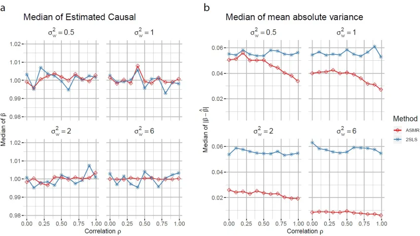
nsim= 1000 simulations ofn= 1000 individuals. Data is generated from distribution (2.6-2.8). In each simulation setting, we varied the confounding effectρfrom 0 (no confounding) to 1 (fully confounded). Across simulation settings, we change the strength of instruments
by varying the mean and variance of dosage,µw andσ2wand the results are shown in Figure
2-3.
We changed the strength of instrument by varying the mean of dosage µw (Figure 2a and
variance of dosageσ2w= 1 and the variance of confounders σv2= 1, σu2 = 1. The strength is considered strong when µw = 6 and µw = 2, and weak when µw = 0.5. We also examined
median strength IV with µw= 1.
Comparing the median of estimated causal effect and true causal effect, in general, 2SLS
and ASMR methods are both approximately unbiased across the range of the confounder
strength ρ. The estimates are more accurate across ρ with stronger instruments (Figure 2b). The stronger the instrument is, the smaller difference between true and estimated
causal effect for both 2SLS and ASMR methods (Figure 2a). When the instrument is weak
(µw = 0.5), ASMR improved the estimation accuracy significantly compared with 2SLS.
The accuracy of ASMR estimation withµw = 0.5 is similar with 2SLS withµw = 1. With
increasing instrument strength (µw = 1,2 and 6), the difference of accuracy between ASMR
and 2SLS becomes smaller. When the instrument is a strong instrument (µw = 6), there is
almost no difference between ASMR and 2SLS. If the strength of instrument is too weak
(µw = 0.2) to explain the gene’s expression levelXor even invalid (µw = 0), the estimation
is unacceptable with large amount of outliers for both 2SLS and ASMR (Figure 17). In
conclusion, when varying the strength of instrument by the mean of dosage, ASMR gives
more accurate estimates of causal effect than 2SLS.
The strength of instrument is determined not only by the mean of dosage, but also by
the variance of dosage σ2w (Equation (2.23)), which determines how much a genotype can explain the true expression level. Two estimation methods are compared by the median
of estimated causal effect ˆβ in Figure 3a. 2SLS and ASMR both give unbiased estimation across different confounder effects when the correlation ρ increases from 0 to 1. We also compared the median absolute difference|βˆ−β|of two methods (Figure 3b). The median absolute differences do not show any change for 2SLS when σ2w increases from 0.5 to 6. This is because the variance of 2SLS estimation is invariant regarding to σw2, wee equation (2.24). However, the median absolute difference for ASMR estimation gets smaller as σ2w
Figure 2: Simulation results when changing instrument strength by the mean of dosage
µw. Under each setting, we simulated 1000 times with the range of confounder strength
ρ∈[0,1].
2SLS while whenσ2w = 6, the median absolute difference of ASMR is about 0.01, which is much lower than that of 2SLS, which is around 0.06. If the variance is smaller, σw2 = 0.2, or even no variation for dosage σw2 = 0, there are barely no difference between ASMR and 2SLS estimates (Figure 3).
In short, the results from simulations show that when the instruments are too weak to
explain the gene’s expression level or when the instruments are very strong, ASMR performs
similarly to 2SLS. When the instruments are weak and can only partially explain the gene’s
expression level, the ASMR has higher power than 2SLS.
2.5. Real data example: Finding downstream targets of lincRNA
Long intergenic non-coding RNAs (lincRNAs) have gained widespread attention in recent
years as a potentially new and crucial layer of biological regulation. lincRNAs of all kinds
have been implicated in a range of developmental processes and diseases, but knowledge of
Figure 3: Simulation results when changing instrument strength by the variance of dosage
σw2. Under each setting, we simulated 1000 times with the range of confounder strength
ρ∈[0,1].
that lincRNAs regulate the transcription of other genes and their mRNA expression. The
causal relations between lincRNAs and mRNAs from coding-genes have been examined in
Mendelian randomization by McDowell et al. (2016) using 2SLS, where they found
signif-icant pairs of lincRNAs and genes. For more information, see recent review by Mattick
(2018). In this section, we applied the allele specific model to real data of lincRNA and
mRNA expression, estimated causal effects by ASMR and 2SLS. We also tested the
signif-icant pairs of lincRNAs and genes from estimated causal effects with empirical variances
and false discovery rate (FDR) control.
2.5.1. Data processing
The raw data is from Geuvadis samples (Lappalainen et al., 2013), filtered by
Hardy-Weinberg equilibrium and read strand bias. There are 87 individuals available in this
dataset. Each individual has 1513 lincRNAs expressions with their tagging SNPs’ genotypes
measured by Fragments Per Kilobase of transcript per Million (FPKM). The expressions of
lincRNAs are measured by read counts and the allele specific information of the lincRNA
expressions are available for heterozygous individuals with respect to the tagging SNPs.
The total expressions are obtained by adding allele specific expressions together. Gene
expressions are measured by FPKM on 26144 non-zero genes.
We selected desirable SNPs before estimating causal effect to save computing time. SNPs
that: (i) can observe 3 genotypes across individuals; (ii) have over 30% of heterozygous;
(iii) have at least one non-zero heterozygous read counts; (iv) have at least one non-zero
homozygous read counts; will be chosen. After filtering, there are 321 SNPs left.
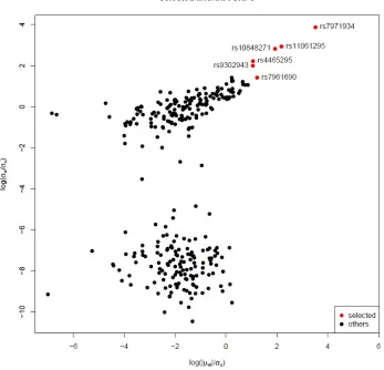
Based on concentration parameter (equation (2.23)) and simulation results, with fixed σu,
larger µw and σw lead to more accurate estimation of causal effect β. Before estimating
causal effect from full likelihood model, we first estimate σu, µw and σw by maximizing
likelihood of model (2.3). We selected genes that are strong instruments based the ratio of
estimatedσw/σuandµw/σu(Figure 4). There are 6 SNPs that shows both largeµw/σuratio
and σw/σu ratio and are considered as strong instruments. The allele specific information
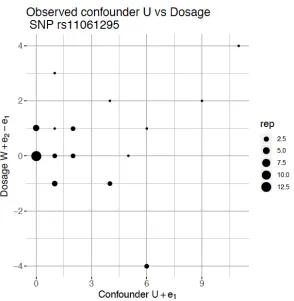
provided by heterozygous individuals allows us to partially check the independence between
confounder U and dosage W by looking at the the allele specific expression from different genotypes. Assume Xi1 and Xi2 are the observed expressions for genotype Zi1 = 0 and
Zi2 = 1 of individuali. Xi1 =Ui+ei1 andXi2−Xi1 =Wi(2)+ei2−ei1 can be viewed as an
approximation of confounderUi and dosageWi(2). We can checked the correlation between
Xi1 and Xi2−Xi1 for the independence of confounderU and dosageW from heterozygous
individuals. As an example, we checked SNP rs11061295 in Figure 5 and the Spearman
correlation betweenXi1 andXi2 is 0.0096.
2.5.2. Estimation of causal effect
We estimate the causal effect as well as other parameters by ASMR from log-likelihoods
Figure 4: Estimated log(|µw|/σu) and log(σw/σu) from first stage likelihood of model (2.3).
Figure 5: Scatter plot of Xi1 vs. Xi2−Xi1 for SNP rs11061295 with heterozygous
and it is compared with ASMR results. To detect reliable causal relation between the
lo-calizable exposure and gene expression, we compare the causal effect estimated by 2SLS
( ˆβ2SLS) and ASMR ( ˆβASM R) after filtering out ASMR results that does converge. In
addi-tion to ˆβ2SLSand ˆβASM R, we also calculated the standard deviation of ˆβASM Rby the Fisher
information matrix (see Section 2.3.2), denoted as sd( ˆβASM R), under the null hypothesis,
where there is no causal effect between lincRNA expression and gene expression. We also
calculated the standard deviation of ˆβ2SLS from equation (2.24), denoted as sd( ˆβ2SLS).
The z-values from ASMR and 2SLS are calculated by zASM R = ˆβASM R/sd( ˆβASM R)and
z2SLS = ˆβ2SLS/sd( ˆβ2SLS) respectively. If we assume standard normality for z2SLS and
zASM R, we will reject the genes that have z-values greater than qnorm(0.975) or less than
qnorm(0.025) for the null hypothesis and consider those genes with real causal effect from ASMR or from 2SLS. Since we are testing 26144 genes at once, we need to control for false
discovery rate (FDR) for multiple testing. We calculated the empirical null distributions
for the z-values from both ASMR and 2SLS and adjusted for multiple testing. Then, for
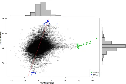
both methods, we select significant genes with reject level α = 0.05. Across 6 candidate SNPs, we focus on genes that are have large z-values from ASMR or 2SLS.
Here we also take SNP rs11061295 as an example. The allele specific information allows us
to partially check the independence between the After adjusted by empirical null, there are
296 genes that are significant differ from zero from ASMR and 1975 genes from 2SLS where
22 of them are also significant from ASMR. We first plot the z-values from estimated causal
effects and standard deviations by 2SLS and ASMR (Figure 6). After adjusted by empirical
null, we selected 20 genes that are uniquely selected by ASMR or 2SLS. From the analysis
and simulations above, we are expected to select more significant genes from ASMR because
it estimates causal effect β more accurately with stronger instruments. Since both 2SLS and ASMR are unbiased methods for estimating causal effect, we are also expected to see a
overlap between significant genes selected by ASMR and 2SLS. However, in this example,
we did not see both patterns. Take a closer look at the expression of SNP as well as the
the z-values from ASMR with empirical null distribution with larger variance. Even though
the 2SLS significant genes have similar z-values from ASMR and 2SLS, the large dispersion
from ASMR empirical null distribution leads to the overlook from ASMR. The significant
genes from ASMR are with extremely high z-values while the 2SLS provides z-values that
are close to zero. This is not because that the actual estimated causal effect from ASMR
ˆ
βASM R is larger than that from 2SLS ˆβ2SLS, in fact, they are similar, but because that the
calculated standard deviation from ASMR are extremely small.
2.6. Conclusion
Mendelian randomization (MR) has been widely studied for estimate causal effect between
gene’s expression level and phenotype of interest. Two-stage least square regression, with
DNA-variants as instruments, is the classical method for MR. In this article, we look for
a new method, ASMR, that can accommodate the development of sequencing techniques
that produced allele-specific data. Maximum likelihood estimation, i.e., estimating every
pa-rameters including the one of interests under the normal assumption, has better estimation
power than classical two stage least squares (2SLS) that ignores allele specific information.
This new method incorporates the allele-specific expression in heterozygous individuals by
separating expression Xi1 and Xi2 in distribution. It would be of interest for future study
CHAPTER 3 : Bulk tissue deconvolution with single cell RNA sequencing
3.1. Introduction
Bulk tissue RNA-seq is a widely adopted method to understand genome-wide transcriptomic
variations in different conditions such as disease states. Bulk RNA-seq measures the average
expression of genes, which is the sum of cell type-specific gene expression weighted by
cell type proportions. Knowledge of cell type composition and their proportions in intact
tissues is important, because certain cell types are more vulnerable for disease than others.
Characterizing the variation of cell type composition across subjects can identify cellular
targets of disease, and adjusting for these variations can clarify downstream analysis.
The rapid development of single-cell RNA-seq (scRNA-seq) technologies have enabled cell
type-specific transcriptome profiling. Although cell type composition and proportions are
obtainable from scRNA-seq, scRNA-seq is still costly, prohibiting its application in clinical
studies that involve a large number of subjects. Furthermore, scRNA-seq is not well suited
to characterizing cell type proportions in a solid tissue, because the cell dissociation step is
biased towards certain cell types (Park et al., 2018).
Computational methods have been developed to deconvolve cell type proportions using cell
type-specific gene expression references (Park et al., 2018). CIBERSORT (Newman et al.,
2015), based on support vector regression, is a widely used method designed for microarray
data. More recently, BSEQ-sc (Baron et al., 2016) extended CIBERSORT to allow the
use of scRNA-seq gene expression as a reference. TIMER (Li et al., 2016), developed
for cancer data, focuses on the quantification of immune cell infiltration. These methods
rely on pre-selected cell type-specific marker genes, and thus are sensitive to the choice of
significance threshold. More importantly, these methods ignore cross-subject heterogeneity
in cell type-specific gene expression as well as within-cell type stochasticity of single-cell gene
expression, both of which cannot be ignored based on our analysis of multiple scRNA-seq
Here we introduce a new MUlti-Subject SIngle Cell deconvolution (MuSiC) method (code
available) that utilizes cross-subject scRNA-seq to estimate cell type proportions in bulk
RNA-seq data. Through comprehensive benchmark evaluations, and applications to
pan-creatic islet and whole kidney expression data in human, mouse, and rats, we show that
MuSiC outperformed existing methods, especially for tissues with closely related cell types.
3.2. Methods
3.2.1. Method overview
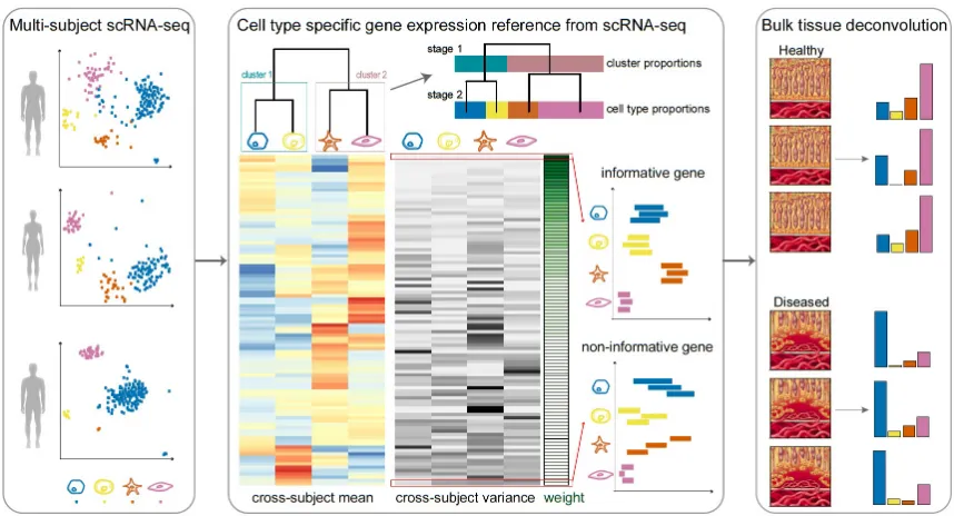
An overview of MuSiC is shown in Figure 7. MuSiC starts with multi-subject scRNA-seq
data, and assumes that the cells for each subject have been classified into a set of fixed
cell types that are shared across subjects. MuSiC deconvolves bulk RNA-seq samples to
obtain the proportions of these cell types in each sample. A key concept in MuSiC is marker
gene consistency. We show that, when using scRNA-seq data as a reference for cell type
deconvolution, two fundamental types of consistency must be considered: cross-subject and
cross-cell, in which the first is to guard against bias in subject selection, and the second is to
guard against bias in cell capture in scRNA-seq. By incorporating both types of consistency,
MuSiC allows for scRNA-seq datasets to serve as effective references for independent bulk
RNA-seq datasets involving different individuals.
Rather than pre-selecting marker genes from scRNA-seq based only on mean expression,
MuSiC gives weight to each gene, allowing for the use of a larger set of genes in
decon-volution. The weighting scheme prioritizes consistent genes across subjects: up-weighing
genes with low cross-subject variance (informative genes) and down-weighing genes with
high cross-subject variance (non-informative genes). This requirement on cross-subject
consistency is critical for transferring cell type-specific gene expression information from
one dataset to another.
Solid tissues often contain closely related cell types, and correlation of gene expression
Figure 7: Overview of MuSiC framework.
proportions in bulk data. To deal with collinearity, MuSiC employs a tree-guided procedure
that recursively zooms in on closely related cell types. Briefly, we first group similar cell
types into the same cluster and estimate cluster proportions, then recursively repeat this
procedure within each cluster (Figure 7). At each recursion stage, we only use genes that
have low within-cluster variance, a.k.a. the cross-cell consistent genes. This is critical as
the mean expression estimates of genes with high variance are affected by the pervasive bias
in cell capture of scRNA-seq experiments, and thus cannot serve as reliable reference.
3.2.2. MuSiC model set-up
In this section, we derive the relation ship between gene expression in bulk tissue and cell
type-specific gene expression in single cells. This relationship forms the basis of our
decon-volution procedure. For geneg, letXjg be the total number of mRNA molecules in subject
j of the given tissue, which is composed of K cell types. Then Xjg = PKk=1Pc∈Ck
j Xjgc,
whereXjgc is the number of mRNA molecules of genegin cell cof subjectj, andCjkis the
set of cell index for cell typek in subjectj withmk
j =|Cjk|being the total number of cells
in this set. The relative abundance of gene gin subjectj for cell typek is
θkjg=
P
c∈Ck
j Xjgc
P
c∈Ck j
PG
g0=1Xjg0c
. (3.1)
We can show that
Xjg= K
X
k=1
mkjSjkθjgk =mj K
X
k=1
pkjSjkθjgk, (3.2)
where for subjectj,Sjk=
P
c∈Ck j
PG g0=1Xjg0c
mk j
is the average number of total mRNA molecules
for cells of cell type k (also referred as “cell type” below), mj = PKk=1mkj is the total
number of cells in the bulk tissue, and pkj = m
k j
mj is the proportion of cells from cell types.
Let Yjg = PGXjg g0=1Xjg0
be the relative abundance of gene g in the bulk tissue of subject j. Equation (3.2) implies
Yjg ∝ K
X
k=1
Thus, acrossG genes in subjectj, we have
Yj1
.. . Yjg ∝
θ1j1 · · · θjK1
..
. . .. ...
θjG1 · · · θjgK
·
Sj1 0 . ..
0 Sjk
·
p1j
.. .
pKj
(3.4)
The goal of MuSiC is to estimate pkj using data from scRNA-seq and bulk RNA-seq.
3.2.3. Model assumptions
If scRNA-seq were available for subjectj, we would be able to obtain the cell size factorSjk
(or the relative values of Sjk, see below) and cell type-specific relative abundance θjgk. With bulk RNA-seq data in subject j, we get the bulk tissue relative abundance Yjg, and, ifθkjg
and Sjk were known, we would be able to perform a regression to estimate pkj. However, since scRNA-seq is still costly, most studies cannot afford the sequencing of a large number
of individuals using scRNA-seq. To make deconvolution possible for a broader range of
studies, it is desirable to utilize cell type-specific gene expression from other studies or from
a smaller set of individuals in the same study. This is feasible under the following three
assumptions:
Assumption 3.1 Individuals with scRNA-seq and bulk RNA-seq are from the same
pop-ulation, with their cell-type specific relative abundances θkjg in equation (3.1) following the same distribution with meanθgk and variance σ2gk,
θjgk ∼F(θkg, σ2gk). (3.5)
Here,F(·,·) represents a general distributional function, which is not assumed to be of any particular form. Under this assumption, deconvolution can use available single-cell data
from other subjects or even subjects from other studies as reference.