IJEDR1904095 International Journal of Engineering Development and Research (www.ijedr.org) 529
Developing a Rapid Curvature Based Data
Reduction Algorithm
1Mohamed Hanafy, 2Ahmed Abdelhafiz, 3Youssef abbbas 1Engineer, 2Professor, 3Professor
1Civil Engineering, Assuit University, Egypt, 2Civil Enginering, Taif University, KSA, 3Civil Engineering, Assuit University, Egypt
_____________________________________________________________________________________________________
Abstract - Nowadays, there is a big demand to create 3D digital models for historical places. Huge point clouds have to
be reduced wisely to enable meshes generation. Reduction algorithms are used to achieve point clouds with reasonable number of points correctly covers all sites features. The meaning here of the correct points coverage is to be dense at curved regions and distant at plane ones. The state-of-the–art curvature algorithm is time consuming. In this work, a new Rapid Curvature based Data Reduction (RCDR) algorithm is developed to reduce large point clouds rapidly and accurately. The comparison between the developed algorithm and the curvature algorithm shows a 5% reduction in accuracy and a huge amount of time saving in the RCDR algorithm. The point cloud, that takes about 36 hours processing time using the curvature algorithm, takes about 11 minutes using the developed one. So, one can fairly see the efficiency of the developed algorithm.
keywords - Point Cloud, Data Acquisition, Data Reduction, K-nearest points, Curvature
_____________________________________________________________________________________________________
1. Introduction
The technology of Laser Scanning (LS) has been widely used in spatial information acquisitions. It provides a decision basis for the Reverse Engineering-RE, Traditional Architecture-TA, Digital City-DC, Cultural Relics-CR protection and complex terrain mapping. Point clouds delivered by LS contain a huge number of points. Such data needs massive storage space. It is also hard to be processed. Therefore, to retain objects features, only useful points of the 3D model have to be preserved. The reduction of the point cloud enhances the data processing speed and efficiency that ensure the final geometric model accuracy. Different methods of sampling and reduction were developed by scholars and experts. These methods classified into two categories, which are; mesh-based reduction and point-based reduction.
Mesh-based reduction method is classified into four main algorithms which are sampling, decimation, vertex merging and adaptive subdivision [1]. It has been then extended to include the energy function optimization [2], [3], [4]. The simplification process is always adjusted using defined metrics. The metrics are divided into global and local classes according to the measured feature. In order to preserve local features, local properties are used as the base of most of the developed metrics [5]. In all mesh-based reduction methods, the mesh is firstly created to show the connectivity between the points. The main advantage of creating meshes first is that they can be used to easily identify nearest points and to realize local continuous surface patches. On the other hand, the main disadvantage of the mesh based method is the high computational cost of mesh generation. It is also quite difficult and sometimes impossible to generate a mesh for a point cloud with millions of points even by employing the latest hardware [6]
Point reduction methods consider the surrounding points in the point cloud to avoid the mesh generation computational cost. It can be classified into three main methods, which are uniform, grid and curvature reduction. Details on the three methods are given in the next paragraphs.
Uniform reduction method tries to equalize the spacing between the points to make the point cloud homogenous. Herráez [7] presented an algorithm to deliver a homogenous distribution point cloud by dividing it into cubes. The cube side length is assumed according to the required sampling percent. The algorithm deletes then the points which are close to the cube centre. The points which appear at adjacent cubes edges are deleted considering certain tolerance. Another two uniform reduction methods utilize distance distributions are introduced by Eetu Puttonen [8] which are the levelled histogram sampling method and the inversely weighted distance sampling method. The levelled histogram sampling method divides the point cloud into groups according to the distances from the scanner. Each group is presented into a histogram. The number of points in each histogram is then calculated. The algorithm equalizes then the number of points in every histogram by deleting points from the group with the large number of points. The inversely weighted distance sampling method sorts also the points according to their distances from the scanner. It evaluates the weight of points according to both the distances from the scanner and the number of points at the same distance from the scanner. The points with low weights are deleted. New weights are then calculated and all the steps are repeated again. The uniform algorithm reduces the point clouds in just few seconds but it deletes easily important features from the model.
IJEDR1904095 International Journal of Engineering Development and Research (www.ijedr.org) 530 consideration. The distance between the two curves at every point is then computed. The point will be deleted if this distance is lower than a certain tolerance. The grid method is computationally inexpensive but it doesn’t consider the curvature on the other direction so many featured points can be deleted. For instance, if a cylinder is considered, the gird algorithm will show low performance, as the points will have low curvature in one direction and high curvature in the other.
Curvature reduction method considers the curvature of the points in more than one direction. Hong Jiang [10] employs the curvature algorithm using the neighbourhood searching method. The algorithm calculates the curvature between each point and the neighbourhood points by using matrices. The Gaussian curvature coefficient, which is equal to (1/radius of curvature)2, is calculated. The points with lower curvature are then deleted. Xiaolei Du [11] computes the normal of the tangent plane after constructing the data topology. The curvature is estimated here using a parabolic fitting method. The normal of every point is then calculated according to the nearest points. The point will be deleted If the normal of the tangent planes are nearly parallel. Guigang Shi [12] estimates the curvature of energy function to build a neighbourhood point set using the KDTree algorithm. The neighbourhood point set is fitted with an osculating sphere. The curvature for the points is calculated to estimate the average value of mean curvatures of the point cloud. The point cloud is then divided into sub-cubes and the average mean curvature for each is estimated. The points in sub-cubes which have mean curvature lower than the average mean curvature are finally deleted. Although the curvature reduction algorithm saves most of the point cloud features, it is a very computational expensive method. In the following section, a new developed algorithm for data reduction is presented. The main characteristics of the new algorithm is that it is computational inexpensive. In the next section, the algorithm has been validated and the results are analysed using real data. Finally, the conclusions are written.
2. Rapid Curvature based Data Reduction (RCDR) algorithm:
An effective algorithm for point cloud reduction should be smart which means that it has the ability to recognize the point cloud features that enables deleting many (un-useful) points in plane areas and fewer points in curved (featured) areas within a reasonable time. The RCDR algorithm is therefore developed to make a smart reduction for LS point clouds considering the curvature in both vertical and horizontal directions. At the same time, the algorithm is not computationally expensive.
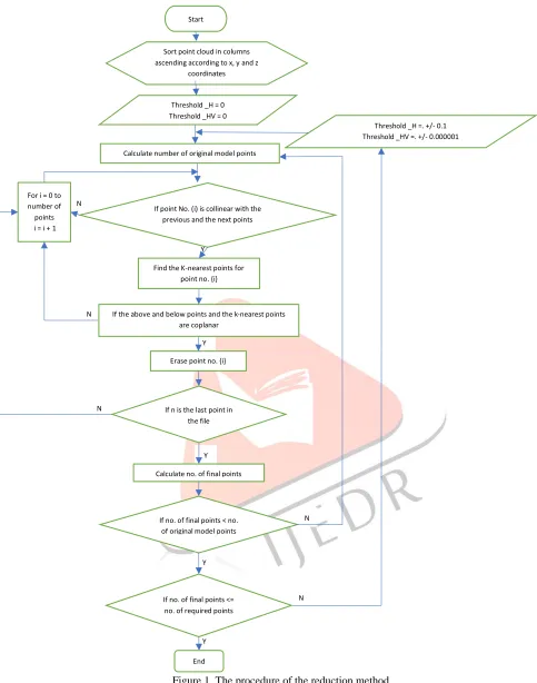
A flowchart for the developed RCDR algorithm is depicted in Figure 1 which, is then coded in C#. The main steps of the algorithm are:
1. Sort the point cloud into columns
2. Check the curvature between the points column by column 3. Searching the k-nearest points
IJEDR1904095 International Journal of Engineering Development and Research (www.ijedr.org) 531 Figure 1. The procedure of the reduction method
2.1. Sort the point cloud into columns
The output data of laser scanners is dense and unstructured and that makes it is time consuming to search for the neighbouring points for every point. The points are therefore sorted here according to their x-coordinates, then according to y-coordinates, followed by z- coordinates. So the points are sorted in columns as shown in figure 2. Certain allowance is considered while sorting.
N
Y Y N
Y
Y
N
Y
N
N
End If no. of final points < no.
of original model points
If no. of final points <= no. of required points Erase point no. {i}
Calculate no. of final points If n is the last point in
the file Find the K-nearest points for
point no. {i}
If the above and below points and the k-nearest points are coplanar
For i = 0 to number of points i = i + 1
If point No. (i) is collinear with the previous and the next points Calculate number of original model points
Threshold _H =. +/- 0.1 Threshold _HV =. +/- 0.000001 Start
Sort point cloud in columns ascending according to x, y and z
coordinates
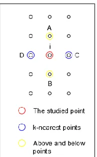
IJEDR1904095 International Journal of Engineering Development and Research (www.ijedr.org) 532 Figure 2. The sorted data shows the studied point (x) in red and the surrounding points
2.2. Check the curvature between the points column by column
In this step, the algorithm checks the curvature for each three points in a column by checking the studied point (i), the above point (A) and the below one (B) as shown in figure 2. Many mathematical equations are used to estimate the curvature between three points in space. Using vectors will accomplish this process quickly. So, vectors have been used to check if the three points lie on one line or not. This can be achieved by calculating two vectors which are; the first vector is from the above point (A) and the below point (B), the other vector is from point (A) and the studied point (i). If the second vector is a multiple of the first one so the three points lie on one line (see equation (1)).
𝐴𝐵
⃑⃑⃑⃑⃑ = 𝑘 𝐴𝑖⃑⃑⃑ (1) Where;
𝐴𝐵
⃑⃑⃑⃑⃑ : Vector between point A and point B 𝐴𝑋
⃑⃑⃑⃑⃑ : Vector between point A and point i 𝑘 : Constant
Equation (1) can be written in the Cartesian coordinate notations as given in equation (2).
(ABx, ABy, ABz) = k (Aix, Aiy, Aiz) (2) Where;
ABx, ABy, ABz: are coordinates for vector ⃑⃑⃑⃑⃑ 𝐴𝐵
Aix, Aiy, Aiz: are coordinates for vector 𝐴𝑖⃑⃑⃑
The following condition should be satisfied in case of the two vectors are collinear:
(Aix / ABx) / (Aiy / ABy) = (Aix / ABx) / (Aiz / ABz) = 1 ± Ԑ1 (3) Where; Ԑ1: Tolerance coefficient (taken 0.1)
If this condition is not true then the three points are not collinear. This means that the point (i) represents a feature in the point cloud. Accordingly it cannot be deleted and there is no need to check the other direction. On the other hand, if the condition is true then the point does not represent a feature in the cloud and it has no value in the vertical direction. So, the algorithm will begin to check the curvature in both the horizontal and the vertical directions simultaneously to investigate if it represents a feature in the plane or not. To make the required check, one should first assign the k-nearest points.
2.3. Searching the k-nearest points
The K-nearest points represent the points which are to the left and to the right of the studied point (i) as shown in figure 2. The traditional method used for searching k-nearest points for point (i) is to calculate all distances from point (i) to all other points in the cloud, then choose the first k nearest points after sorting the distances ascendingly. However, this method is time-consuming and inefficient, especially for point clouds with millions of points. In this algorithm, an improved method is used to find the required k-nearest points. This improved method gets use of the first step of sorting the point cloud. While the required k-nearest left point (D) can be found when moving up into the sorted cloud file, the right k-nearest point (C) is found when moving downwards. The following steps explain the method of execution:
1- To find the left k-nearest point (D); a cube of (s1 = 0.001 m) side length is assumed around the studied point (i).
2- Search for a point lies inside the assumed cube. This can be found by checking the differences of the coordinate’s components between point (i) and the points above it until a point satisfied equations (4, 5, and 6). This point is marked as the left k-nearest point. Otherwise, a point with differences exceeding a value of (s2= 10*s1) in the three components of coordinates is reached then the searching process will stop.
XD – Xi = +/- 0.5 * s1 (4) YD – Yi = +/- 0.5 * s1 (5) ZD – Zi = +/- 0.5 * s1 (6) Where;
XD, YD, ZD: are coordinates of point D Xi, Yi, Zi: are coordinates for point i
IJEDR1904095 International Journal of Engineering Development and Research (www.ijedr.org) 533 4- If no point satisfied the required conditions, the side length of the assumed cube is increased automatically by a value equal to (d1=0.001 m).
5- To find the right k-nearest point (C), all the previous steps are repeated with the points downwards in the sorted point cloud file.
2.4. Check simultaneously the curvature in both of the horizontal and the vertical directions.
After catching the previous two k-nearest points, the four points (A&B&C&D) are to be checked with point (i). State-of-the-art methods estimate the curvature between the checked point and the surrounding points. In this work, the mode around the checked point is tested. If the mode is plane then the checked point will be deleted otherwise the checked point will remain in the cloud. The main advantage of this method is that it is computationally inexpensive.
The following steps are followed to perform this check: i. Try to fit a plane with the four points (A&B&C&D).
ii. If the four points cannot form one plane then the mode around the checked point is curved, so, leave point (i) in the point cloud.
iii. If the four points can form one plane, then the mode around the checked point is plane. So, the checked point (i) can be removed safely from the point cloud.
The four points (A&B&C&D) will form a plane if they satisfy the following equation (7).
𝐴𝐵
⃑⃑⃑⃑⃑ . [𝐴𝐶⃑⃑⃑⃑⃑ 𝑥 𝐴𝐷⃑⃑⃑⃑⃑ ] = 0 ± Ԑ2 (7) Where;
𝐴𝐵
⃑⃑⃑⃑⃑ : Vector between point A and point B 𝐴𝐶
⃑⃑⃑⃑⃑ : Vector between point A and point C 𝐴𝐷
⃑⃑⃑⃑⃑ : Vector between point A and point D
Equation (7) can be written in the Cartesian coordinate notations as given in equations (8) and (9).
𝐴𝐵
⃑⃑⃑⃑⃑ . [𝐴𝐶⃑⃑⃑⃑⃑ 𝑥 𝐴𝐷⃑⃑⃑⃑⃑ ] = |𝐴𝐵𝑥𝐴𝐶𝑥 𝐴𝐵𝑦𝐴𝐶𝑦 𝐴𝐵𝑧𝐴𝐶𝑧
𝐴𝐷𝑥 𝐴𝐷𝑦 𝐴𝐷𝑧
| (8)
|
𝐴𝐵𝑥 𝐴𝐵𝑦 𝐴𝐵𝑧
𝐴𝐶𝑥 𝐴𝐶𝑦 𝐴𝐶𝑧
𝐴𝐷𝑥 𝐴𝐷𝑦 𝐴𝐷𝑧
| = 𝐴𝐵𝑥 |𝐴𝐷𝑦𝐴𝐶𝑦 𝐴𝐷𝑧𝐴𝐶𝑧| − 𝐴𝐵𝑦 |𝐴𝐶𝑥 𝐴𝐶𝑧
𝐴𝐷𝑥 𝐴𝐷𝑧| + 𝐴𝐵𝑧 |
𝐴𝐶𝑥 𝐴𝐶𝑦
𝐴𝐷𝑥 𝐴𝐷𝑦| = 0 ± Ԑ2 (9)
Where;
Ԑ2: Tolerance coefficient taken equal to 0.000001 3. Validating the developed RCDR algorithm.
In order to validate the developed RCDR algorithm, the main three methods of data reduction are applied on a real historical site in comparison with the RCDR. The Uniform, Grid, and Curvature algorithms, which are available in the GEOMAGIC STUDIO commercial Software, are the three main methods applied. The curvature algorithm is considered here as the reference reduction algorithm.
3.1 The selected historical site
In this work, the Baron Empain’s Palace was taken as the case study. It was built by Baron-General Edouard Louis Joseph Empain in the period between 1907 and 1911 in Heliopolis, Cairo Egypt. The palace is considered one of the most famous buildings in Cairo so that it was annexed to the tourism sector (Figure 3).
The scanned data was obtained as a result of collaboration between two Egyptian Universities and Vienna University. About fifty students with their supervisors participated to a workshop on city analysis and building archaeology, focused on scanning the Baron Palace and its urban surroundings.
Figure 3. Baron Palace, Heliopolis, Cairo Egypt 3.2 Data capturing
IJEDR1904095 International Journal of Engineering Development and Research (www.ijedr.org) 534 Figure 4. The used z+f laser scanner.
3.3 Data reduction and analysis
After capturing the site, two test clouds from the palace point cloud including curved and plane areas were selected. While the first part (a terrace of the Baron palace) has only about 1 million points (Figure 5), the second one (the front view of the palace) has about 9 million points (Figure 6).
Figure 5. A terrace of the Baron palace Figure 6. The front view of the Baron palace
The three reduction algorithms as well as the developed one were applied in each part. Afterwards, a mesh model was created for each reduced cloud as a reference model. Each mesh is compared with the original mesh to obtain the areas of errors. The average error, the maximum error, the standard deviation, and the total value of errors were then calculated. The total value of error represents here the summation of all errors existed in all the points in the reduced cloud in respect to the original mesh. This value is used to evaluate the accuracy of each reduction algorithm. The time required for each reduction process is also computed.
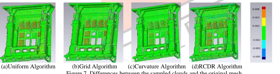
Figure 7 shows the differences between the sampled cloud and the original mesh using a color chart. While the red and blue zones reflect big differences, the green zones reflect accepted differences (+/- 5mm).
(a)Uniform Algorithm (b)Grid Algorithm (c)Curvature Algorithm (d)RCDR Algorithm Figure 7. Differences between the sampled clouds and the original mesh
Table 1 and Table 2 show the obtained numerical differences results for the two selected clouds. The average positive and negative errors using the four algorithms in both clouds are approximately the same. The maximum error has millimetres fluctuating differences between the algorithms. The standard deviation is slightly raised in the uniform and grid algorithm comparing to the curvature and the RCDR. The differences are clearly appeared in the total value of error.
Table 1. A comparison between Uniform, Grid, RCDR and curvature algorithms for the first part. Unifor
m Grid
Curvatur
e RCDR
Average Distance (m)
Positive 0.0021 0.0021 0.0021 0.0021 Negative -0.0022 -0.0022 -0.0021 -0.0021
Maximum Distance (m)
Positive 0.331 0.331 0.3175 0.3078 Negative -0.3175 -0.3076 -0.3135 -0.3201 Standard Deviation (m) 0.0041 0.0039 0.0036 0.0037
IJEDR1904095 International Journal of Engineering Development and Research (www.ijedr.org) 535 Table 2. A comparison between Uniform, Grid, RCDR and curvature algorithms for the second part .
Uniform Grid Curvature RCDR
Average Distance
Positive 0.003 0.0029 0.0029 0.0029 Negative -0.0031 -0.0030 -0.0029 -0.0030 Maximum Distance Positive 0.5230 0.5121 0.5072 0.5135 Negative -0.5092 -0.5227 -0.5013 -0.5007 Standard Deviation 0.0052 0.0050 0.0046 0.0047 Value of errors 236.609 218.758 185.157 193.295 Time consuming 5 min 7 min 960 min 9 min
From Table 1, the total value of error shows that the curvature algorithm has the best performance. The RCDR has an increase of 5.6% in the total error comparing to 17.4% and 29.7% increase in the total error for the grid and the uniform algorithms respectively. The required time to achieve the reduction is seconds in all cases.
From Table 2, the total value of error shows also that the curvature algorithm has the best performance. The RCDR has an increase of 4.4% in the total error comparing to 18.2% and 27.8% increase in the total error for the grid and the uniform algorithms respectively. On the other hand, the time required for reduction (about 16 hours) shows the superiority of the RCDR algorithm. The curvature algorithm requires 107 times the time required by the RCDR algorithm.
Considering the reduction in the accuracy in the RCDR algorithm (4% - 5%) and the very high performance in speed comparing to the curvature algorithm, one can fairly vote for the RCDR algorithm especially in the large data manipulation projects.
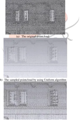
Figure 8-e shows the effective behaviour of the RCDR algorithm as it recognizes the surfaces with lower curvature and deleted more points in them. On contrarily, it keeps the points in the surface with high curvature (Feature regions).
(a) The original pointcloud
(b) The sampled pointcloud by using Uniform algorithm
IJEDR1904095 International Journal of Engineering Development and Research (www.ijedr.org) 536 (d) The sampled pointcloud by using Curvature algorithm
(e) The sampled pointcloud by using RCDR algorithm
Figure 8. Difference between original pointcloud and sampled one by using the four algorithms
A whole point cloud with about 18 million points is also reduced using the RCDR algorithm. It takes about 11 minutes to be accomplished. The same point cloud takes about 36 hours processing time by the curvature algorithm using the same hardware (see figure 9). Due to technical issues, it is impossible to generate a mesh using the 18 million points with the recent available hardware in order to compute the total value of error in each case. This is again proves the efficiency of the developed algorithm and the need for such reduction algorithm.
(a) The sampled pointcloud by using Curvature algorithm (b) The sampled pointcloud by using RCDR algorithm Figure 9. Difference between original pointcloud and sampled one by using the RCDR and Curvature algorithms 4. Conclusion
IJEDR1904095 International Journal of Engineering Development and Research (www.ijedr.org) 537 REFRENCES
1. Luebke, D.P., A developer's survey of polygonal simplification algorithms. IEEE Computer Graphics and Applications, 2001. 21(3): p. 24-35.
2. Cignoni, P., C. Montani, and R. Scopigno, A comparison of mesh simplification algorithms. Computers & Graphics, 1998. 22(1): p. 37-54.
3. Hoppe, H. Progressive meshes. in Proceedings of the 23rd annual conference on Computer graphics and interactive techniques. 1996. ACM.
4. Klein, R., G. Liebich, and W. Straßer. Mesh reduction with error control. in Proceedings of Seventh Annual IEEE Visualization'96. 1996. IEEE.
5. Tang, H., et al., Moment-based metrics for mesh simplification. Computers & Graphics, 2007. 31(5): p. 710-718.
6. Han, H., et al., Point cloud simplification with preserved edge based on normal vector. Optik-International Journal for Light and Electron Optics, 2015. 126(19): p. 2157-2162.
7. Herraez, J., et al., Optimal modelling of buildings through simultaneous automatic simplifications of point clouds obtained with a laser scanner. Measurement, 2016. 93: p. 243-251.
8. Puttonen, E., et al., Improved sampling for terrestrial and mobile laser scanner point cloud data. Remote Sensing, 2013. 5(4): p. 1754-1773.
9. Wang, Y.-Q., et al., A simple point cloud data reduction method based on Akima spline interpolation for digital copying manufacture. The International Journal of Advanced Manufacturing Technology, 2013. 69(9-12): p. 2149-2159.
10. Jiang, H., et al., A study and implementation on the data reduction based on the curvature of point clouds.
11. Du, X. and Y. Zhuo. A point cloud data reduction method based on curvature. in 2009 IEEE 10th International Conference on Computer-Aided Industrial Design & Conceptual Design. 2009. IEEE.