https://doi.org/10.5194/os-14-453-2018
© Author(s) 2018. This work is distributed under the Creative Commons Attribution 4.0 License.
Numerical modeling of surface wave development under
the action of wind
Dmitry Chalikov1,2,3
1Shirshov Institute of Oceanology, Saint Petersburg 199053, Russia
2Russian State Hydrometeorological University, Saint Petersburg 195196, Russia 3University of Melbourne, Victoria 3010, Australia
Correspondence:Dmitry Chalikov ([email protected]) Received: 31 January 2018 – Discussion started: 20 February 2018
Revised: 21 April 2018 – Accepted: 10 May 2018 – Published: 11 June 2018
Abstract.The numerical modeling of two-dimensional sur-face wave development under the action of wind is per-formed. The model is based on three-dimensional equations of potential motion with a free surface written in a surface-following nonorthogonal curvilinear coordinate system in which depth is counted from a moving surface. A three-dimensional Poisson equation for the velocity potential is solved iteratively. A Fourier transform method, a second-order accuracy approximation of vertical derivatives on a stretched vertical grid and fourth-order Runge–Kutta time stepping are used. Both the input energy to waves and dis-sipation of wave energy are calculated on the basis of earlier developed and validated algorithms. A one-processor version of the model for PC allows us to simulate an evolution of the wave field with thousands of degrees of freedom over thousands of wave periods. A long-time evolution of a two-dimensional wave structure is illustrated by the spectra of wave surface and the input and output of energy.
1 Introduction
The phase-resolving modeling of sea waves is the mathemat-ical modeling of surface waves including explicit simulations of surface elevation and a velocity field evolution. As com-pared with spectral wave modeling, phase-resolving model-ing is more general since it reproduces a real visible physi-cal process and is based on well-formulated full equations. Phase-resolving models usually operate with a large num-ber of degrees of freedom. In general, this method is more complicated and requires more computational resources. The
with no periodicity the problem becomes more complicated since the Fourier presentation cannot be used directly.
From the point of view of physics, the problem of phase-resolving modeling can be divided into two groups: the adi-abatic and nonadiadi-abatic modeling. A simple adiadi-abatic model assumes that the process develops with no input or output of energy. Being not completely free of limitations, such a formulation allows the investigation of the wave motion on the basis of true initial equations. Including the effects of in-put energy and its dissipation is always connected with the assumptions that generally contradict the assumption of po-tentiality, i.e., the new terms added to the equations should be referred to as pure phenomenological. This is why the treat-ment of a nonadiabatic approach is often based on quite dif-ferent constructions.
All of the phase-resolving models use the methods of com-putational mathematics and inherit all their advantages and disadvantages; i.e., on the one side, there is the possibility of a detailed description of the processes, and on the other side, there are a bunch of the specific problems connected with the computational stability, space and time resolution. The mathematical modeling produces tremendous volumes of in-formation, the processing of which can be more complicated than the modeling itself.
The phase-resolving wave modeling takes a lot of com-puter time since it normally uses a surface-following coordi-nate system, which considerably complicates the equations. The most time-consuming part of the model is an elliptic equation for the velocity potential usually solved with iter-ations. Luckily, for a two-dimensional problem this trouble is completely eliminated by use of the conformal coordi-nates, reducing the problem to a one-dimensional system of equations which can be solved with high accuracy (Chalikov and Sheinin, 1998). For a three-dimensional problem, the re-duction to a two-dimensional form is evidently impossible; hence, the solution of a 3-D elliptical equation for the veloc-ity potential becomes an essential part of the entire problem. This equation is quite similar to the equation for pressure in a nonpotential problem. It follows that the 3-D Euler equa-tions, being more complicated, can still be solved over the acceptable computer time.
There is a large volume of papers devoted to the numerical methods developed for the investigation of wave processes over the past decades. It includes a finite-difference method (Engsig-Karup et al., 2009, 2012), a finite-volume method (Causon et al., 2010), a finite-element method (Ma and Yan, 2010; Greaves, 2010), a boundary (integral) element method (Grue and Fructus, 2010), and spectral methods (Ducroset et al., 2007, 2012, 2016; Touboul and Kharif, 2010; Bon-nefoy et al., 2010). These include a smoothed-particle hy-drodynamics method (Dalrymple et al., 2010), a large-eddy simulation (LES) method (Issa et al., 2010; Lubin and Cal-tagirone, 2010), a moving particle semi-implicit method (Kim et al., 2014), a constrained interpolation profile method (Zhao, 2016), a method of fundamental solutions (Young et
al., 2010) and a meshless local Petrov–Galerkin method (Ma and Yan, 2010). A fully nonlinear model should be applied to many problems. Most of the models were designed for engineering applications such as overturning waves, broken waves, waves generated by landslides, freak waves, solitary waves, tsunamis, violent sloshing waves, an interaction of ex-treme waves with beaches and an interaction of steep waves with the fixed structures or with different floating structures. The references given above make up less than 1 % of the pub-lications on those topics.
A two-dimensional approach (like a conformal method) considers a strongly idealized wave field since even monochromatic waves in the presence of lateral disturbances quickly obtain a two-dimensional structure. The difficulty arising is not a direct result of the increase in the dimen-sion. The fundamental complication is that the problem can-not be reduced to a two-dimensional problem, and even for the case of a double-periodic wave field, the problem of so-lution of a Laplace-like equation for the velocity potential arises. The majority of the models designed for investigation of the three-dimensional wave dynamics are based on simpli-fied equations such as the second-order perturbation methods in which the higher-order terms are ignored. Overall, it is un-clear which effects are missing in such simplified models.
The most sophisticated method is based on the full three-dimensional equations and surface integral formulations (Beale, 2001; Xue et al., 2001; Grilli et al., 2001; Clamond and Grue, 2001; Clamond et al., 2005, 2006; Fructus et al., 2005; Guyenne et al., 2006; Fochesato et al., 2006). A fully nonlinear model of three-dimensional water waves, which extends an approach suggested by Craig and Sulem (1993), was originally given in a two-dimensional setting. The model is based upon the Hamiltonian formulation (Zakharov, 1968), which allows the reduction of the problem of surface variable computation by introducing a Dirichlet–Neumann operator, which is expressed in terms of its Taylor series expansion in homogeneous powers of surface elevation. Each term in this Taylor series can be obtained from the recursion formula and efficiently computed using a fast Fourier transform.
freely responding floating structures (Liu et al., 2016; Gou et al., 2016).
However, the BIEM seems to be quite complicated and time consuming when applied to the long-term evolution of a multimode wave field in large domains. The simulation of the relatively simple wave fields illustrates an application of the method, and it is unlikely that the method can be applied to the simulation of the long-term evolution of a large-scale multimode wave field with a broad spectrum. An implemen-tation of a multipole technique for a general problem of the sea wave simulation (Fochesato et al., 2006) can solve the problem but obviously leads to considerable algorithmic dif-ficulties.
Currently, the most popular approach in the oceanogra-phy approach is a HOS (high-order scheme) model devel-oped by Dommermuth and Yue (1987) and West et al. (1987). The HOS model is based on a paper by Zakharov (1968) in which a convenient form of the dynamic and kinematic sur-face conditions was suggested. The equations used by Za-kharov were not intended for modeling, but rather for inves-tigation of stability of the finite amplitude waves. In fact, a system of coordinates in which depth is counted from the surface was used, but the Laplace equation for the veloc-ity potential was taken in its traditional form. However, the Zakharov’s followers have accepted this idea literally. They used the two coordinate systems: a curvilinear surface-fitting system for the surface conditions and the Cartesian system for calculation of the surface vertical velocity. An analytical solution for the velocity potential in the Cartesian coordinate system is known. It is based on the Fourier coefficients on a fixed level, while the true variables are the Fourier coef-ficients for the potential on a free surface. Here a problem of transition from one coordinate system to another arises. This problem is solved by expansion of the surface poten-tial into the Taylor series in the vicinity of the surface. The accuracy of this method depends on that of the representa-tion of the exponential funcrepresenta-tion with a finite number of the Taylor series. For the small-amplitude waves and for a nar-row wave spectrum, such accuracy is evidently satisfactory. However, for the case of a broad wave spectrum that con-tains many wave modes, the order of the Taylor series should be high. The problem is now that the waves with high wave numbers are superposed over the surface of larger waves. Since the amplitudes of a surface potential attenuate expo-nentially, the amplitude of a small wave at a positive eleva-tion increases, and conversely, it can approach zero at neg-ative elevations. It is clear that such a setting of the HOS model cannot reproduce high-frequency waves, which actu-ally reduces the nonlinearity of the model. This is why such a model can be integrated for long periods using no high-frequency smoothing. In addition, an accuracy of the calcu-lation of a vertical velocity on the surface depends on full elevation at each point. Hence, the accuracy is not uniform along the wave profile. A substantial extension of the Taylor series can definitely result in numerical instability due to the
occasional amplification of modes with high wave numbers. The authors of a surface integral method share a similar point of view (Clamond et al., 2005). We should note, however, that the comparison of the HOS method based on the West et al. (1987) approach using a method of the surface integral for an idealized wave field (Clamond et al., 2006) shows quite acceptable results. It was shown in the previous paper that a method suggested by Dommermuth et al. (1987) demon-strates poorer divergence of the expansion for the vertical ve-locity than the method by West et al. (1987). The HOS model has been widely used (for example, Tanaka, 2001; Toffoli et al., 2010; Touboul and Kharif, 2010) and it has shown its ability to efficiently simulate the wave evolution (propaga-tion, nonlinear wave–wave interactions, etc.) in a large-scale domain (Ducrozet et al., 2007, 2012). It is obvious that the HOS model can be used for many practical purposes. Re-cently, Ecole Centrale Nantes, LHEEA Laboratory (CNRÑ) announced that the nonlinear wave models based on HOS are published as an open source (https://github.com/LHEEA/ HOS-ocean/wiki, last access: 6 June 2018).
Opposite to the HOS method based on the analytical so-lution of the Laplace equation in Cartesian coordinates, a group of models is based on a direct solution of the equa-tion for the velocity potential in the curvilinear coordinates (Engsig-Karup et al., 2009, 2012; Chalikov et al., 2014). The main advantage of a surface-following coordinate system is that a variable surface is mapped onto the fixed plane. Since the wave motion is very conservative, the highly accurate nu-merical schemes should be used for a good description of the nonlinearity and spectrum transformation. This most univer-sal approach is being developed at the Technical University of Denmark (TUD) (see Engsig-Karup, 2009). Actually, the models ModelWave3D developed at TUD are targeted at the solution of a variety of problems, including such problems as the modeling of wave interaction with submerged objects as well as the simulation of wave regime in basins with a real shape and topography.
OceanWave3D-Open-Source-Marine-Hydrodynamics (last access: 6 June 2018).
A comparison of a ModelWave3D with a HOS model was presented by Ducrozet et al. (2012). It was shown that both models demonstrate high accuracy, while the HOS model shows a better performance. Note that the comparison of the speed of the models in this case is irrelevant since the Model-Wave3D was designed for investigation of complicated pro-cesses, taking into account the real shape of a basin, variable depth and even the presence of engineering constructions. All these features are obviously not included in the HOS model. The development of waves under the action of wind is a process that is difficult to simulate since surface waves are very conservative and change their energy for hundreds and thousands of periods. This is why the most popular method is spectral modeling. Waves as physical objects in this approach are actually absent since an evolution of the spectral distri-bution of wave energy is simulated. The description of in-put and dissipation in this approach is not directly connected with the formulation of the problem, but rather it is adopted from other branches of wave theory in which waves are the objects of investigation. However, the spectral approach was found to be the only method capable of describing the space and time evolution of wave field in the ocean. The phase-resolving models (or “direct” models) designed for reproduc-ing the waves themselves cannot compete with the spectral models since the typical size of the domain in such models does not exceed several kilometers. Such a domain includes just several thousands of large waves. Nevertheless, the direct wave modeling plays an ever-increasing role in geophysical fluid dynamics because it gives the possibility of investigat-ing the processes which cannot be reproduced with spectral models. One such problem is that of an extreme wave gener-ation (Chalikov, 2009; Chalikov and Babanin, 2016a). Direct modeling is also a perfect instrument for the development of parameterization of physical processes for spectral wave models. In addition, such models can be used for direct sim-ulation of wave regimes of small water basins, for example, port harbors. Other approaches of direct modeling are dis-cussed in Chalikov et al. (2014) and Chalikov (2016).
Until recently the direct modeling was used for repro-duction of a quasi-stationary wave regime when the wave spectrum did not change significantly. A unique example of the direct numerical modeling of a surface wave evolution is given in Chalikov and Babanin (2014), in which the de-velopment of a wave field was calculated with the use of a two-dimensional model based on the full potential equa-tions written in the conformal coordinates. The model in-cluded the algorithms for parameterization of the input and dissipation of energy (a description of similar algorithms is given below). The model successfully reproduced an evolu-tion of wave spectrum under the acevolu-tion of wind. However, the strictly one-dimensional (unidirected) waves are not re-alistic; hence, a full problem of wave evolution should be
formulated on the basis of the three-dimensional equations. An example of such modeling is given in the current paper.
2 Equations
Let us introduce a nonstationary surface-following nonorthogonal coordinate system:
ξ=x, ϑ=y, ζ =z−η(ξ, ϑ, τ ), τ =t , (1)
whereη(x, y, t )=η(ξ, ϑ, τ )is a moving periodic wave sur-face given by the Fourier series
η (ξ, ϑ, τ )= X −Mx<k<Mx
X −My<l<My
hk,l(τ ) 2k,l, (2)
wherekandlare the components of a wave number vector k,hk,l(τ ) are Fourier amplitudes for elevations η (ξ, ϑ, τ ), Mx andMy are the numbers of modes in the directionsξ andϑ, respectively, and2k,lare the Fourier expansion basis functions, represented as the matrix
2kl=
cos(kξ+lϑ ) −Mx≤k≤Mx,−My< l <0 cos(kξ ) −Mx≤k≤0, l=0 sin(kξ ) 0≤k≤My, l=0 sin(kξ+lϑ ) −Mx≤k≤Mx,0< l≤My
. (3)
The 3-D equations of potential waves in the system of co-ordinates (1) atζ ≤0 take the following form:
ητ = −ηξϕξ−ηϑϕϑ+
1+η2ξ+η2ϑ8ς, (4) ϕτ= −
1 2
ϕξ2+ϕ2ϑ−1+η2ξ+η2ϑ82ζ−η−p, (5)
8ξ ξ+8ϑ ϑ+8ζ ζ=ϒ (8) , (6)
whereϒis the operator:
ϒ ( )=2ηξ( )ξ ζ+2ηϑ( )ϑ ζ+ ηξ ξ+ηϑ ϑ( )ζ−
ηξ2+η2ϑ( )ζ ζ. (7)
Capital fonts8are used for domainζ <0 while the lower caseϕ refers to ζ=0. A term p in Eq. (5) described the pressure on the surfaceζ=0.
It is suggested in Chalikov et al. (2014) that it is con-venient to represent the velocity potential ϕ as a sum of two components, i.e., an analytical (linear) component
¯
8 ϕ¯= ¯8 (ξ, ϑ,0)
and an arbitrary (nonlinear) component
e
8 eϕ=8 (ξ, ϑ,e 0)
:
ϕ=ϕ+
e
ϕ, 8=8+8.e (8)
The analytical component8¯ satisfies the Laplace equation ¯
8ξ ξ+ ¯8ϑ ϑ+ ¯8ζ ζ=0, (9)
with a known solution: ¯
8(ξ, ϑ, ζ, τ )=X k,l
¯
(where|k| = k2+l21/2andϕ¯k,lare the Fourier coefficients of a surface analytical potentialϕ¯atζ=0). The solution sat-isfies the following boundary conditions:
ς=0: 8¯ = ¯ϕ ς→ −∞ : e8ζ→0
. (11)
The nonlinear component satisfies an equation:
e
8ξ ξ+e8ϑ ϑ+e8ζ ζ =ϒ 8e
+ϒ 8¯. (12) Equation (12) is solved with the boundary conditions
ς=0: e8=0 ς→ −∞ : e8ζ→0
. (13)
The derivatives of a linear component 8¯ in Eq. (7) are calculated analytically. The scheme combines a 2-D Fourier transform method in the “horizontal surfaces” and a second-order finite-difference approximation on a stretched stag-gered grid defined by the relation 1ζj+1=χ 1ζj (1ζ is a vertical step, while j=1 at the surface). A stretched grid provides an increase in accuracy of approximation for the exponentially decaying modes. The values of a stretching coefficient χ lie within the interval 1.01–1.20. A finite-difference second-order approximation of the vertical opera-tors in Eq. (12) on a nonuniform vertical grid is quite straight-forward. Equation (12) is solved as the Poisson equations with the iterations over the right-hand side. At each time step, the iterations start with the right-hand side calculated at the previous time step. The initial elevation was generated as a superposition of linear waves corresponding to a JONSWAP spectrum (Hasselmann et al., 1973) with random phases. The initial Fourier amplitudes for the surface potential were cal-culated using the formulas of the linear wave theory. A de-tailed description of the scheme and its validation is given in Chalikov et al. (2014) and Chalikov (2016).
Equations (4)–(6) are written in a nondimensional form by using the following scales: lengthLwhere 2π Lis a (dimen-sional) period in the horizontal direction, timeL1/2g−1/2and the velocity potentialL3/2g1/2(gis an acceleration of grav-ity). The pressure is normalized by water density, so that the pressure scale isLg. Equations (4)–(6) are self-similar to the transformation with respect to L. The dimensional size of the domain is 2π L, so the scaled size is 2π. All of the re-sults presented in this paper are nondimensional. Note that the number of the Fourier modes can be different in the x
andydirections. In this case it is assumed that the two-length scalesLxandLyare used. The nondimensional length of the domain in the y direction remains equal to 2π and a factor
r=Lx/Lyis introduced into the definition of a differential operator in the Fourier space.
3 Energy input and dissipation
The energy input to waves is described by a pressure termp
in a dynamic boundary condition (Eq. 5). The tangent stress
on the surface cannot be taken into account in the potential formulation. The dissipation cannot be described either with use of the potential equations, but for a realistic description of wave dynamics, the dissipation of wave energy should be taken into account, i.e., we should include additional terms in Eqs. (4) and (5), which, strictly speaking, contradict an assumption of potentiality.
3.1 Energy input from wind
According to the linear theory (Miles, 1957), the Fourier components of surface pressurepare connected with those of the surface elevation through the following expression:
pk,l+ip−k,−l= ρa ρw
βk,l+iβ−k,−l hk,l+ih−k,−l, (14) wherehk,l, h−k,−l, βk,l, β−k,−lare real and imaginary parts of elevationηand the so-calledβ function (i.e., Fourier co-efficients at COS and SIN, respectively);ρa/ρwis a ratio of the air and water densities. Equation (14) is a standard pre-sentation of pressure above a multimode surface. It means that every wave mode with amplitudeh2k,l+h2−k,−l
1/2 ini-tiates the pressure mode with amplitudep2k,l+p2−k,−l1/2
shifted off the phase of a wave mode by angleα=atanβ−k,−l
βk,l .
third-generation wave forecast model (Tolman and Chalikov, 1996), and thoroughly validated against the experimental data in the course of developing WAVEWATCH III (Tolman et al., 2014). This method was later improved on the basis of a more advanced coupled modeling of waves and boundary layer (Chalikov and Rainchik, 2010), while the β function used in WAVEWATCH III was corrected and extended up to the high frequencies. A direct calculation of the energy in-put to waves requires both the real and imaginary parts of theβ function. The total energy input to waves depends on an imaginary part of theβ function, while the moments of a higher order depend on both the imaginary and real parts of
β. This is why a full approximation constructed in Chalikov and Rainchik (2010) was used in the current work. Note that in a range of relatively low frequencies the new method is very close to the scheme implemented in WAVEWATCH III. It is a traditional suggestion that both coefficients are the functions of the virtual nondimensional frequency=
ωk,lUcosψ=U/ck,lcosψ(whereωk,landUare the nondi-mensional radian frequency and wind speed, respectively;
ck,l is a phase speed of the kth mode; ψ is an angle be-tween the wind and wave mode directions). Most of the schemes for calculations of the β function consider a rela-tively narrow interval of the nondimensional frequencies. In the current work, the range of frequencies cover an in-terval(0< <10), and occasionally the values of >10 can appear. This is another reason why the function derived in Chalikov and Rainchik (2010) through the coupled sim-ulations of waves and the boundary layer is used here. The wave model is based on the potential equations for a flow with a free surface, extended with an algorithm for the break-ing dissipation (see below a description of the breakbreak-ing dis-sipation parameterization). The wave boundary layer (WBL) model is based on Reynolds equations closed with aK−ε
scheme; the solutions for air and water are matched through the interface. Theβ function was used for the evaluation of accuracy of the surface pressure p calculations. The shape of theβ function connecting surface elevations and surface pressure is studied up to the high nondimensional wave fre-quencies in both positive and negative (i.e., for wind oppo-site to waves) domains. The data on theβ function exhibit wide scatter, but since the volume of the data was quite large (47 long-term numerical runs allowed us to generate about 1 400 000 values ofβ), the shape of theβ function was de-fined with satisfactory accuracy up to the very high nondi-mensional frequencies(−50< <50). As a result, the data on theβ-function in such a broad range allow us to calculate the wave drag up to very high frequencies and to explicitly divide the fluxes of energy and momentum transferred by the pressure and molecular viscosity. This method is free of arbi-trary assumptions on a drag coefficientCd, and, conversely, such calculations allow the investigation of the nature of the wave drag (see Ting et al., 2012).
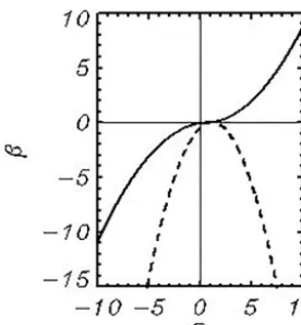
The most reliable data onβ function are concentrated in the interval−10< <10 (negative values ofcorrespond
to the wave modes running against wind). The real and imag-inary parts of theβ function are shown in Fig. 1. It is a cor-rected version of an approximation given in Chalikov and Rainchik (2010) in which the data at negative were in-terpreted erroneously. In the current calculations the modes running against wind are absent. The functionβ can be ap-proximated by the formulas
βk,l=
β0+a0(−0)+a1(−0)2 0<
β0+a0(−0)−a1(−0)2 < 0
, (15)
β−k,−l= ( β
1+a3(−2) < 2
a2(−1)2 2< < 3
β1−a3(−3) 3<
, (16)
where the coefficients are a1=0.09476, a2= −0.3718, a3=14.80, β0= −0.02, β= −148. a0= 0.02277, 0=0.02277, 1=1.20, 2= −18.8, 3= 21.2.
It was indicated above that an initial wave field is assigned as a superposition of linear modes whose amplitudes are cal-culated with a JONSWAP spectrum with an initial peak wave numberkp0=100. An initial valueU/cp0=6 was chosen, i.e., a ratio of the nondimensional wind speed at the height of one-half the initial peak wave lengthλ0/2=2π/100, and the phase speedcp0=kp0
−1/2
is equal to 6. Such a high ratio corresponds to the initial stages of wave development. The wind velocity 6c0p remains constant throughout the integra-tion. The values offor other wave numbers are calculated by assuming that the wind profile is logarithmic:
k,l= U ck,l
lnλk,l 2z0
ln λ0 2z00
−1
cosψk,l, (17)
wherez00 is an effective nondimensional roughness for the initial wind profile, whilez0is an actual roughness parame-ter that depends on the energy in a high-frequency part of the spectrum and on the wind profile. We call it “effective” since very close to the surface the wind profile is not logarithmic (Chalikov, 1995; Tolman and Chalikov, 1996; Chalikov and Rainchik, 2010). The value of this parameter depends on the wind velocity and energy in a high-wave-number interval of the wave spectrum, as well as on the length scale of the prob-lem. All these effects are possible to include by matching the wave model with a one-dimensional WBL model (Ting et al., 2012). Here, a simplified scheme for the roughness parame-ter is chosen. It is well known that the roughness parameparame-ter (as well as a drag coefficient) increases with a decrease in the inverse wave age. In our case the wind speed is fixed, and de-pendence for a nondimensional roughness parameter is con-structed on the basis of the results obtained in Chalikov and Rainchik (2010):
z0=15z00, (18)
Figure 1.Real (dashed curve) and imaginary (solid curve) parts of theβfunction.
the results are not sensitive to the variation of the roughness parameter within reasonable limits.
3.2 High-wave-number energy dissipation
A nonlinear flux of energy directed to the small wave num-bers produces the downshifting of the spectrum, while an opposite flux forms the shape of the spectral tail. The sec-ond process can produce the accumulation of energy near a “cut” wave number. Both processes become more intensive with an increase in the energy input. The growth of ampli-tudes at high wave numbers is followed by that of the local steepness and numerical instability. This well-known phe-nomenon in the numerical fluid mechanics is eliminated by use of a highly selective filter simulating the nonlinear vis-cosity. To support stability, additional terms are included in the right-hand sides of Eqs. (4) and (5):
∂ηk,l
∂τ =Ek,l−µk,lηk,l, (19)
∂ϕk,l
∂τ =Fk,l−µk,lϕk,l. (20)
Ek,landFk,lare the Fourier amplitudes of the right-hand sides of Eqs. (4) and (5) while a factorµk,lis calculated using the formula
µk,l=
0 |k|< kd
cmk0
|k| −k d
(k0−kd) 2
kd≤ |k| ≤k0
cmk0 |k|> k0
, (21)
wherekandlare components of wave number|k|, while the coefficientskdandk0are defined by the expression:
kd=dm2MxMy
l|k|−1dmMx 2
+k|k|−1dmMy 2−1/2
, (22)
k0=MxMy
l|k|−1Mx 2
+k|k|−1My 2−1/2
, (23)
wherecm=0.1 anddm=0.75. The expressions (19)–(21) can be interpreted in a straightforward way: the value of µk,l is equal to zero inside the ellipse with semiaxesdmMx and dmMy; then it grows linearly with |k| up to the value cm and is equal to cm outside the outer ellipse. This method of filtration that we call “tail dissipation” was developed and validated with a conformal model by Chalikov and Sheinin (1998). The sensitivity of the results to the param-eters in Eqs. (21)–(23) is not high. The aim of the algorithm is to support smoothness and monotonicity of the wave spec-trum within a high wave number range. Since the algorithm affects the amplitudes of small modes, it actually does not reduce the total energy, though it efficiently prevents devel-opment of the numerical instability. Note that no long-term calculations can be performed without tail dissipation elimi-nating the development of numerical instability at high wave numbers.
3.3 Dissipation due to wave breaking
The main process of wave dissipation is wave breaking. This process is taken into account in all the spectral wave forecast-ing models similar to WAVEWATCH (see Tolman and Cha-likov, 1996). Since there are no waves in the spectral models, no local criteria of wave breaking can be formulated. This is why the breaking dissipation is represented in spectral mod-els in a distorted form. A real breaking occurs in relatively narrow areas of the physical space; however, a spectral im-age of such breaking is stretched over the entire wave spec-trum, while in reality the breaking decreases height and en-ergy of dominant waves. This contradiction occurs because the waves in spectral models are assumed to be the linear ones, while in fact the breaking occurs in the physical space with a nonlinear sharp wave, usually composed of several modes. However, progress has been gradually made in spec-tral wave modeling over the past decade. It became clear that state-of-the-art wave models should account for the thresh-old behavior of the dominant wave breaking, i.e., waves will not break unless their steepness exceeds the threshold (Alves and Banner, 2003; Babanin et al., 2010).
wave, which becomes sharper and unstable. Probably even more frequent cases of wave breaking and extreme wave ap-pearance can be explained by a local superposition of several modes.
The instability of interface leading to the breaking is an important and poorly developed problem of fluid mechanics. In general, this essentially nonlinear process should be inves-tigated for a two-phase flow. Such an approach was demon-strated, for example, by Iafrati (2009). However, progress in solving this highly complicated problem is slow.
A problem of the breaking parameterization includes two points: (1) establishing of a criterion of the breaking onset and (2) development of an algorithm of the breaking param-eterization. The problem of breaking is discussed in detail in Babanin (2011). Chalikov and Babanin (2012) performed a numerical investigation of the processes leading to the break-ing. It was found that a clear predictor of the breaking for-mulated in dynamical and geometrical terms probably does not exist. The most evident criterion of the breaking is the breaking itself, i.e., the process when some part of the upper portion of a sharp wave crest is falling down. This process is usually followed by separation of the detached volume of liquid into the water and air phases. Unfortunately, there is no possibility of describing this process within the scope of the potential theory.
Some investigators suggest using a physical velocity ap-proaching the rate of surface movement in the same direction as a criterion of the breaking onset. This is incorrect since a kinematic boundary condition suggests that these quantities are exactly equal to each other. It is quite clear that the onset of breaking can be characterized by the appearance of a non-single-value piece of surface. This stage can be investigated with a two-dimensional model, which due to a high flexi-bility of the conformal coordinates allows us to reproduce a surface with an inclination in the Cartesian coordinates ex-ceeding 90 degrees. (In the conformal coordinates the depen-dence of elevation on a curvilinear coordinate is always a sin-gle value). The duration of this stage is extremely short, the calculations being always interrupted by the numerical insta-bility with sharp violation of the conservation laws (constant integral invariants, i.e., full energy and volume) and strong distortion of the local structure of flow. The numerous numer-ical experiments with a conformal model showed that after the appearance of a non-single value the model never returns to stability. However, the introduction of a non-single surface as a criterion of the breaking instability even in a conformal model is impossible since a behavior of the model at a critical point is unpredictable, and the run is most likely to be termi-nated, no matter what kind of parameterization of breaking is introduced. It means that even in a precise conformal model the stabilization of the solution should be initiated prior to the breaking.
A consideration of an exact criterion for the breaking on-set for the models using transformation of the coordinate type of point (1) is useless since the numerical instability in such
models arises not because of the approach of breaking but be-cause of the appearance of large local steepness. The multiple experiments with a direct 3-D wave model show that the ap-pearance of the local steepness max(∂η/∂x, ∂η/∂y) exceed-ing≈2 (that corresponds to a slope of about 60 degrees) is always followed by the numerical instability but the instabil-ity can happen well before reaching this value. The decrease in a time step does not make any effect. As seen, a surface with such a slope is very far from being a vertical wall, when the real breaking starts. However, an algorithm for the break-ing parameterization must prevent numerical instability. The situation is similar to the numerical modeling of turbulence (LES technique) in which a local highly selective viscosity is used to prevent the appearance of too large local gradients of the velocity. A description of the breaking in the direct wave modeling should satisfy the following conditions. (1) It should prevent the onset of instability at each point of half a million grid points over more than 100 thousand time steps. (2) It should describe in a more or less realistic way the loss of kinetic and potential energies with preservation of balance between them. (3) It should preserve the volume. It was sug-gested in Chalikov (2005) that an acceptable scheme can be based on a local highly selective diffusion operator with a special diffusion coefficient. Several schemes of such type were validated, and finally the following scheme was cho-sen:
ητ =Eη+J−1
∂
∂ξBξ ∂η
∂ξ + ∂
∂ϑBϑ ∂η
∂ϑ
, (24)
ϕτ=Fϕ+J−1
∂
∂ξBξ ∂ϕ ∂ξ +
∂ ∂ϑBϑ
∂ϕ ∂ϑ
, (25)
whereFη andFϕ are the right-hand sides of Eqs. (4) and (5) including the terms introduced in terms of Fourier coef-ficients by Eqs. (19)–(23);Bξ andBϑ are diffusion coeffi-cients. It was suggested in the first versions of the scheme that a diffusion coefficient depends on a local slope; how-ever, such a scheme did not prove to be very reliable since it did not prevent all of the events of the numerical instability. A scheme based on the calculation of the local curvilinearity
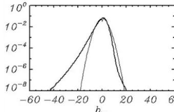
ηξ ξ andηϑ ϑ turned out to be a lot more robust. The calcu-lations of 75 different runs were performed with a full 3-D model in Chalikov et al. (2014) over the period oft=350 (70 000 time steps). The total number of values used for the calculations of dependence in Fig. 2 (thick curve) is about 6 billion. The normal probability calculated with the same dispersion is shown by a thin curve.
It is seen that the probability of large negative values of the curvilinearity is calculated over an ensemble of linear modes by orders larger than the probability with the spectra gener-ated by a nonlinear model.
Figure 2.Probability of the curvilinearityηξ ξ. The thick curve is calculated with a full 3-D model; the thin curve is the probability calculated over an ensemble of linear modes with the same spec-trum.
nonlinearly on the curvilinearity:
Bξ=
1ξ CBη2ξ ξ ηξ ξ< ηξ ξcr 0 ηξ ξ≥ηξ ξcr
, (26)
Bϑ=
1ϑ C
Bη2ϑ ϑ ηϑ ϑ< ηcrξ ξ 0 ηϑ ϑ≥ηcrξ ξ
, (27)
where 1ξ and 1ζ are the horizontal steps in thex and y
directions in a grid space, and the coefficients areCB=2.0 and ηcrξ ξ=ηcrϑ ϑ= −50. Equations (24)–(27) do not change the volume and decrease the local potential and kinetic en-ergy. It is assumed that the lost momentum and energy are transferred to the current and turbulence (see Chalikov and Belevich, 1992). In addition, the energy also goes to other wave modes. The choice of parameters in Eqs. (24)–(27) is based on simple considerations: a local piece of surface can closely approach the critical curvilinearity but not exceed it. The values of the coefficients are picked with reserve to pro-vide stability for long runs.
We do not think that the suggested breaking parameteri-zation is a final solution to the problem. Other schemes will be tested in the next version of the model. However, the re-sults presented below show that the scheme is reliable and provides a realistic energy dissipation rate.
4 Calculations and results
The elevation and surface velocity potential fields are ap-proximated in the current calculations by Mx=256 and My=128 modes in directions x and y. The correspond-ing grid includes Nx×Ny=(1024×512)knots. The ver-tical derivatives are approximated at a verver-tical stretched grid
dζj+1=χ dζj, (j =1,2,3. . ., Lw), whereν=1.2 andLw= 10. A small number of levels used for the solution of the equation for a nonlinear component of the velocity potential are possible because just a surface vertical derivative for the velocity potential ∂8/∂ζ (ζ=0) is required. The velocity potential mainly consists of an analytical componentϕ¯, while
a nonlinear component provides only a small correction. To reach the accuracy of the solutionε=10−6for Eq. (11), no more than two iterations were usually sufficient.
The parameters chosen were used for solution of a prob-lem of a wave field evolution over the acceptable time (of the order of 10 days). The initial conditions were assigned on the basis of the empirical spectrum JONSWAP (Hasselmann et al., 1973) with a maximum placed at the wave number
kp=100 with the angle spreading(coshψ )256. The details of the initial conditions are of no importance because an ini-tial energy level is quite low.
The total energy of a wave motionE=Ep+Ek(Epis a potential energy, whileEkis a kinetic energy) is calculated with the following formulas:
Ep=0.25η2, Ek=0.5
ϕ2
x+ϕy2+ϕz2
, (28)
where a single bar denotes averaging over theξ andϑ coor-dinates, and a double bar denotes averaging over the entire volume. The derivatives in Eq. (25) are calculated according to the transformation (1). An equation of the integral energy
E=Ep+Ekevolution can be represented in the following form:
dE
dt =I+Db+Dt+N , (29)
whereI is the integral input of energy from wind (Eqs. 14– 18);Dbis the rate of the energy dissipation due to the wave breaking (Eqs. 24–27);Dtis the rate of the energy dissipa-tion due to filtradissipa-tion of high-wave-number modes (tail dissi-pation, Eqs. 19–23);N is an integral effect of the nonlinear interactions described by the right-hand side of the equations when the surface pressurepis equal to zero. The differential form for calculation of the energy transformation can be, in principle, derived from Eqs. (4)–(6), but here a more conve-nient and simple method was applied. Different rates of the integral energy transformations can be calculated with the help of fictitious time steps (i.e., apart from the basic cal-culations). For example, the value ofI is calculated by the following relation:
I= 1
1t
Et+1t−Et
, (30)
whereEt+1t is the integral energy of a wave field obtained after one time step with the right side of Eq. (6) contain-ing only the surface pressure calculated with Eqs. (14)–(18). For calculation of the dissipation rate due to filtration, the right-hand side of the equations contains just the terms intro-duced in Eqs. (19)–(23), while for calculation of the effects of breaking, only the terms introduced in Eqs. (24)–(27) are in use.
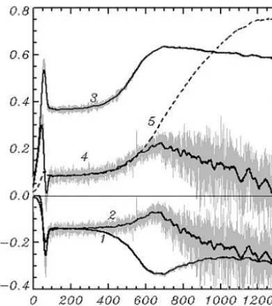
Figure 3.Evolution of integral characteristics of the solution, a rate of evolution of the integral energy multiplied by 107due to 1 – tail dissipationDt(Eqs. 19–23), 2 – breaking dissipationDb(Eqs. 24– 27), 3 – input of energy from windI(Eqs. 14–18) and 4 – balance of energyI+Dt+Db. Curve 5 shows the evolution of wave energy 105E. Grey vertical bars show the instantaneous values; the thick curve shows the smoothed behavior.
initial linear fields to the nonlinearity. Up to the end of inte-gration, the sum of all energy transition terms (tail dissipation
Dt, breaking dissipationDband energy inputI )approaches zero (curve 4), and the energy growthE(curve 5) stops. Then the energy tends to decrease, but we are not sure about the na-ture of this effect. Such behavior can be explained by a fluc-tuating character of mutual adjustment of input and dissipa-tion or simply by deterioradissipa-tion of the approximadissipa-tion because of the downshifting process. Note that opposite to a more or less monotonic behavior of the tail dissipation (curve 1), the breaking dissipation is highly intermittent, which is consis-tent with the common views on the wave breaking nature.
The data on the evolution of the wave spectrum are shown in Fig. 4. A 2-D wave spectrum S(k, l)
0≤k≤Mx,−My≤l≤Myaveraged over 13 time inter-vals of length equal to 1t≈100 was transferred to the polar coordinatesSp(ψ, r) (−π/2≤ψ≤π/2,0≤r≤Mx) and then averaged over the angleψto obtain a 1-D spectrum
Sh(r): Sh(r)=
X
Sp(ψ, r) r1ψ. (31)
An angleψ=0 coincides with the direction of windU,
1ψ=π/180.
Figure 4.The wave spectraSh(r)integrated over angleψin the po-lar coordinates and averaged over the consequent intervals of length for about 100 units of the nondimensional timet. The spectra grow and shift from right to left.
As seen, each spectrum consists of separated peaks and holes1. This phenomenon was first observed and discussed by Chalikov et al. (2014). The repeated calculations with different resolution showed that such a structure of the 2-D spectrum is typical. It cannot be explained by a fixed com-bination of interacting modes since in different runs (with the same initial conditions but a different set of phases for the modes) the peaks are located at different locations in a Fourier space.
Another presentation is given in Fig. 6 in which the log10(S (ψ, r)), averaged over the successive seven-period length1t=200, is given. The first panel with a mark of 0 refers to the initial conditions. The disturbances within the range (125< k <150) reflect the initial adjustment of input and dissipation at a high-wave-number slope of spectrum. The pictures characterize the downshifting and angle spread-ing of the spectrum well due to the nonlinear interactions.
Evolution of the integrated-over-anglesψwave spectrum
Sh(r)can be described with the equation dSh(r)
dt =I (r)+Dt(r)+Db(r)+N (r), (32)
whereI (r) , Dt(r) , Db(r)andN (r) are the spectra of the input energy, tail dissipation, breaking dissipation and the rate of the nonlinear interactions, all obtained by integration over anglesψ. All of the spectra shown below were obtained by transformation of the 2-D spectra into a polar coordinate
(ψ, r)and then integrated over anglesψwithin the interval
Figure 5.Sequence of 3-D images of lg10(S (k, l)), in which each panel corresponds to a single curve in Fig. 3. The left side refers to the wave numberl −My≤l≤Myand the front side refers to k (0≤k≤M). The numbers indicate the end of the time interval expressed in hundreds of nondimensional time units.
example, a spectrum of the energy inputI (k, l)is calculated as follows:
I (k, l)= Sct+1t(k, l)−Sct(k, l)
/1t, (33)
whereSc kx, ky
is the spectrum of the columnar energy cal-culated by the relation
Sc(k, l)= 1 2
h2k,l+h2−k,−l+ 0
Z
−H
(u2k,l+u2−k,−l+vk,l2 +v2−k,−l+wk,l2 +w2−k,−l)dζ,
(34) where the grid values of velocity componentsu, vandware calculated by the relations
u=ϕξ+ϕζηξ, v=ϕϑ+ϕζηϑ, w=ϕζ, (35) anduk,l, vk,landwk,lare their Fourier coefficients.
For calculation ofI (k, l)the fictitious time steps1t are made only with a term responsible for the energy input, i.e.,
Figure 6.Sequence of 2-D images of lg10(S(k, l))averaged over the consequent seven periods of length1t=200. The numbers in-dicate the period of averaging (first panel marked 0, refers to the initial conditions). The horizontal and vertical axes correspond to the wave numberskandl, respectively.
surface pressurep. A spectrumI (k, l)was averaged over the periods1t≈100, then transformed into a polar coordinate system and integrated in a Fourier space over anglesψwithin the interval(−π/2, π/2) .
Evolution of the input spectra (Fig. 7) is in general similar to that of the wave spectra shown in Fig. 4. Note that the maximum of the spectra is located at the maximum of the wave spectra since the input depends mainly on the spectral density, while the dependence on frequency is less important. An algorithm (Eq. 30) was applied for calculation of the dissipation spectra due to dumping of a high-wave-number part of spectrum (tail dissipation) and for calculation of the spectrum of the breaking dissipation. In the first case, the fictitious time step was made taking into account the terms described by Eqs. (19)–(23), while in the second case the time step was made using the terms described by Eqs. (24)– (27).
The spectra of the tail dissipation calculated similarly to the spectraI (r)are shown in Fig. 8. The dissipation occurs at the periphery of the spectrum, outside an ellipse with semi-axesdmMx anddmMy2. This is why such dissipation, aver-aged over angles, seems to affect the middle part of a 1-D spectrum. The tail dissipation effectively stabilizes the solu-tion.
Figure 7.The spectrum of energy inputI (r)integrated over angle ψ in the polar coordinates and averaged over the consequent inter-vals of length for about 100 units of the nondimensional timet.
Figure 8.The tail dissipation spectraDt(r)integrated over angleψ in the polar coordinates and averaged over the consequent intervals of length for about 100 units of the nondimensional timet.
The breaking dissipation averaged over angles is presented in Fig. 8. As seen, the breaking dissipation has a maximum at the spectral peak. This does not mean that in the vicin-ity of the wave peak the probabilvicin-ity of large curvilinearvicin-ity is quite high. A high rate of the breaking dissipation can be explained by high wave energy in the vicinity of the wave peak. The energy lost through the breaking, described by the diffusion mechanism, correlates with the energy of breaking waves. Opposite to the high-wave-number dissipation which regulates the shape of the spectral tail, the breaking dissipa-tion forms the main energy-containing part of the spectrum.
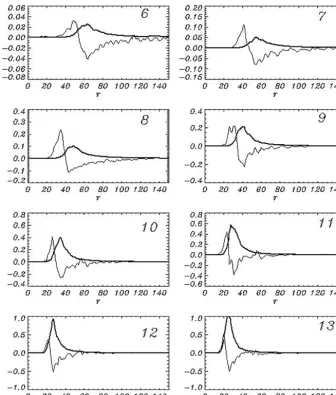
The diffusion mechanism suggested in Eqs. (24)–(27) modifies an elevation and surface stream function in close vicinity of the breaking point. The amplitudes of side per-turbation are small and decrease very quickly throughout the distance from the breaking point.
An example of the profile of the energy input due to the breakingDb(x)is given in Fig. 10. As seen, the energy in-put fluctuates around the breaking point. A diffusion operator
Figure 9.The breaking dissipation spectraDb(r)integrated over angleψin the polar coordinates and averaged over the consequent intervals of length for about 100 units of the nondimensional time t.
chosen for the breaking parameterization not only decreases total energy but also redistributes the energy between Fourier modes in a Fourier space.
In general, for the specific conditions considered in this paper, the breaking is an occasional process taking place in a small part of the domain. The kurtosis of the input energy due to the breakingDb(ξ, ϑ ), i.e., the value
Ku=Db4
Db2 −2
−3, (36)
is of the order of 103, which corresponds to a plain function with occasional separated peaks.
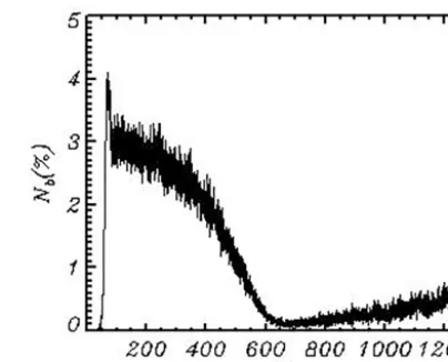
The number of breaking points in terms of percentage of the total number of points is given in Fig. 11. As seen, the number of breaking events decreases tot=600 and then in-creases till the end of the calculations. The number of break-ing events is not directly connected with the intensity of breaking, which is seen when comparing Fig. 11 and curve 2 in Fig. 3.
Figure 10.Example of the energy input due to the breakingDb(x).
(downshifting). Opposite to the Hasselmann’s theory, these results are obtained by solution of the full three-dimensional equations. It would be interesting to compare our results with the calculations of Hasselmann’s integral. Unfortunately, nei-ther of the existing programs of such a type permits cal-culations with the high resolution that was used in the cur-rent model. Note that the nonlinear interactions also produce widening of the spectrum.
As can be seen, the nonlinearity is quite an important prop-erty of surface waves. The contribution of nonlinearity can be estimated, for example, by comparison of the kinetic energy of a linear componentEl=0.5
¯
ϕ2
x+ ¯ϕ2y+ ¯ϕz2
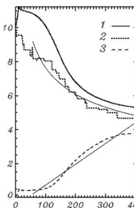
and the total kinetic energyEk(Fig. 13). A ratioEl/Ekas a function of time remains very close to 1, which proves that the nonlinear part of energy makes up just a small percentage of the total energy. It does not mean that the role of the nonlinearity is small; its influence can manifest itself over large timescales. The time evolution of the integral spectral characteristics is presented in Fig. 14. Curve 1 corresponds to the weighted frequencyωw
ωw=
RkSdkdl R
Sdkdl 1/2
, (37)
where integrals are taken over the entire Fourier domain. The valueωwis not sensitive to the details of the spectrum; hence, it characterizes the position of spectrum and its shifting well. Curve 2 describes an evolution of the spectral maximum. The step shape of the curve corresponds to the fundamental prop-erty of downshifting. Opposite to the common views, the de-velopment of spectrum occurs not monotonically but by the appearance of a new maximum at a lower wave number as well as by attenuation of the previous maximum. It is inter-esting to note that the same phenomenon is also observed in a spectral model (Rogers et al., 2012). Curve 3 describes the change of total energyE=Ep+Ek. As seen, all three curves have a tendency to slow down the evolution rate. Then the en-ergy tends to decrease, but we are not sure about the nature of this effect. Such behavior can be explained by a fluctuat-ing character of mutual adjustment of input and dissipation or simply by deterioration of the approximation because of the downshifting process. The numerical experiment repro-duces the case when development of wave field occurs un-der the action of a permanent and uniform wind. This case corresponds to a JONSWAP experiment. Despite large scat-ter, the data allow us to construct empirical approximations of a wave spectrum, as well as to investigate the evolution
Figure 11.Evolution of a number of the wave breaking eventsNb expressed in percentage of the number of grid pointsNx×Ny.
of a spectrum as a function of fetchF. In particular, it is suggested that the frequency of a spectral peak changes as
F−1/3, while the full energy grows linearly withF. Neither of the dependences can be exact since they do not take into account the approach to a stationary regime. In addition, the dependence of frequency on fetch is singular atF =0.
The value of fetch in a periodic problem can be calcu-lated by integration of a peak phase velocity cp= |k|−1/2 over time.
F =
t Z
t0
cpdt (38)
The JONSWAP dependencies for the frequency of a spec-tral peakωpand the full energy Eare shown in Fig. 14 by thin curves. Dependenceωp∼F1/3is qualitatively valid. A dependence of the total energy on fetch does not look like a linear one, but it is worth noting that the JONSWAP de-pendence is evidently inapplicable to a very small and large fetch.
5 Discussion
Figure 12.Sequence of wave spectraSh(r)(thick curves) and a nonlinear input termN (r)(thin curves) averaged over the eight consequent intervals of length1t=100 starting from the sixth period.
Figure 13.Time evolution of the ratioEl/Ek.
the solution of a variety of problems including such problems as the modeling of wave interaction with submerged objects and the simulation of a wave regime in basins with real shape and topography.
In the current paper a three-dimensional model was used for simulation of the development of a wave field under the action of wind and dissipation. The input energy is described
by a single term, i.e., surface pressurepin Eq. (4). It is tra-ditionally assumed that the complex pressure amplitude in a Fourier space is linearly connected with the complex el-evation amplitude through a complex coefficient called the
Figure 14.Time evolution of weighted frequencyωw(1) (Eq. 34), the spectral peak frequency ωp=k1p/2 (2) and full energyE(3) (Eq. 28). Thin curves correspond to the empirical dependences for the peak wave number and energy.F is a distance passed by the spectral peak.
We are not familiar with any observational data that can be used for the formulation of a statistically provided scheme for calculation of the input energy to waves. The only method that can give more or less reliable results is the mathematical modeling of the statistical structure of a turbulent boundary layer above a curvilinear moving surface whose characteris-tics satisfy the kinematic conditions. The method described above is based on several millions of values of the pres-sure referred strictly to the surface. As a whole, the prob-lem of a boundary layer seems even more complicated than the wave problem itself. Some early attempts to solve this problem were made on the basis of a finite-difference two-dimensional model of a boundary layer written in a sim-ple surface following the coordinate (see review Chalikov, 1986). Waves were assigned as a superposition of linear modes with random phases, corresponding to the empirical wave spectrum. This approach was not quite accurate since it did not take into account the nonlinear properties of sur-face (for example, the sharpness of real waves and the ab-sence of a dispersive relation for the waves of medium and high frequencies). The next step was the formulation of cou-pled models for a boundary layer and potential waves, both written in the conformal coordinates (Chalikov and Rainchik, 2010). The calculations showed that the pressure field con-sists mostly of random fluctuations not directly connected with the waves. A small part of these fluctuations are in phase with the surface disturbances. The calculated values ofβ in Eq. (13) have large dispersion. However, since the volume of data was very large, the shape of theβ function was found
with a high level of accuracy. Probably, the approximation of β used in the current work can be considered most ad-equate. We are planning additional investigations based on the coupled wind–wave models. The next step in the inves-tigations of wave boundary layer (WBL) should use a three-dimensional LES approach. Note that even the availability of a large volume of data on the structure of WBL does not make the problem of parameterization of wind input in the spectral wave models easily solvable since the pressure is characterized by a broad continuous spectrum created by nonlinearity.
The wave breaking is obviously even more complicated than the input energy. Nevertheless, this problem can be sim-plified, if the common ideas used in the numerical fluid me-chanics are accepted. For example, in the LES modeling a more or less artificial viscosity is introduced to prevent too large local velocity gradients. In fact the numerical insta-bility terminating computations precedes the wave breaking. Hence, the scheme should prevent the breaking approach to preserve stability of the numerical scheme. Hence, a wave model should contain the algorithms preventing the appear-ance of too large slopes. A criterion of breaking is introduced not for recognizing the breaking itself, but for the choice of places where it might happen (or, unfortunately, might not happen). Finally, the algorithm should produce the lo-cal smoothing of elevation (and the surface potential). The algorithm should be highly selective so that the “breaking” could occur within narrow intervals and not affect the entire area. The exact criteria of the breaking events (most evident of them is the breaking itself) cannot be used for parame-terization of breaking since in a coordinate system (1) the numerical instability occurs long before the breaking. In our opinion, the most sensitive parameter indicating potential in-stability is the curvilinearity (second derivative) of elevation. In the current work, the breaking is parameterized by a diffusion algorithm with a nonlinear coefficient of diffusion providing high selectivity of the smoothing. We admit that such an approach can be realized in many different forms. The same situation is observed in a problem of the turbu-lence modeling for parameterization of subgrid scales. Note that the breaking dissipation in phase-resolving models is in-cluded in a more realistic manner than in spectral models. For example, the breaking is simulated in a physical space, which allows us to reduce the height and energy of the non-linear waves composed of several modes. In spectral models the dissipation is distributed more or less arbitrarily over the entire spectrum. The spectral models sometimes include ad-ditional dissipation of short waves due to their modulation by long waves (Young and Babanin, 2006; Babanin et al., 2010). In the phase-resolving models this process has been included explicitly.
The numerical models of waves similar to that considered in this paper have a lot of important applications. First, they are a perfect tool for the development of physical parame-terization schemes in spectral wave models. Second, a di-rect model can be used in future for the numerical simula-tion of wave processes in the basins of small and medium size. These investigations can be based on the HOS model (Ducrozet et al., 2016) or the model used in the current pa-per. However, the most universal approach seems to be de-veloped at the Technical University of Denmark (see Engsig-Karup, 2009). Any model used for the long-term simulation of wave field evolution should include the algorithms de-scribing transformation of energy similar to those considered in the current paper.
Data availability. The underlying data (150 Gb) are not publicly accessible. Any number of them can be shared upon request.
Competing interests. The authors declare that they have no conflict of interest.
Acknowledgements. The authors thank Olga Chalikova for her assistance in preparation of the paper as well as the anonymous reviewers for their constructive comments. This investigation was supported by Russian Science Foundation, project 16-17-00124.
Edited by: Neil Wells
Reviewed by: two anonymous referees
References
Alberello, A., Chabchoub, A., Monty, J. P., Nelli, F., Lee, J. H., Elsnab, J., and Toffoli, A.: An experimental comparison of ve-locities underneath focused breaking waves, Ocean Eng., 155, 201–210 2018.
Alves, J. H. G. M. and Banner, M. L.: Performance of a Saturation-Based Dissipation-Rate Source Term in Modeling the Fetch-Limited Evolution of Wind Waves, J. Phys. Oceanogr., 33, 1274– 1298, 2003.
Al’Zanaidi, M. A. and Hui, H. W: Turbulent airflow over water waves-a numerical study, J. Fluid Mech., 148, 225–246, 1984. Babanin, A. V., Tsagareli, K. N., Young, I. R., and Walker, D. J.:
Nu-merical Investigation of Spectral Evolution of Wind Waves. Part II: Dissipation Term and Evolution Tests, J. of Phys. Oceanogra-phy, 40, 667–683, 2010.
Babanin, A. V.: Breaking and Dissipation of Ocean Surface Waves, Cambridge University Press, The Edinburgh Building, Cam-bridge, UK, 480 pp., 2011.
Beale, J. T.: A convergent boundary integral method for three-dimensional water waves, Math. Comput., 70, 977–1029, 2001. Bonnefoy, F., Ducrozet, G., Le Touzé, D., and Ferrant,
P.: Time-domain simulation of nonlinear water waves us-ing spectral methods, in: Advances in Numerical
Simu-lation of Nonlinear Water Waves, Advances in Coastal and Ocean Engineering, World Scientific, 11, 129–164, https://doi.org/10.1142/9789812836502_0004, 2010.
Causon, D. M., Mingham, C. G., and Qian, L.: Developments In Multi-Fluid Finite Volume Free Surface Capturing Methods, Ad-vances in Numerical Simulation of Nonlinear Water Waves, 11, 397–427, 2010.
Chalikov, D.: The Parameterization of the Wave Boundary Layer, J. Phys. Oceanogr., 25, 1335–1349, 1995.
Chalikov, D.: Statistical properties of nonlinear one-dimensional wave fields, Nonlinear Proc. Geoph., 12, 1–19, 2005.
Chalikov, D.: Freak waves: their occurrence and probability, Phys. Fluids, 21, 076602, https://doi.org/10.1063/1.3175713, 2009. Chalikov, D.: Numerical modeling of sea waves, Springer
International Publishing AG, Switzerland, 330 pp., https://doi.org/10.1007/978-3-319-32916-1, 2016.
Chalikov, D. V.: Numerical simulation of windwave interaction, J. Fluid. Mech., 87, 561–582, 1978.
Chalikov, D. V.: Numerical simulation of the boundary layer above waves, Bound. Layer Met., 34, 63–98, 1986.
Chalikov, D. and Babanin, A. V.: Simulation of Wave Breaking in One-Dimensional Spectral Environment, J. Phys. Oceanogr., 42, 1745–1761, 2012.
Chalikov, D. and Babanin, A. V.: Simulation of one-dimensional evolution of wind waves in a deep water, Phys. Fluids, 26, 096607, https://doi.org/10.1063/1.4896378, 2014.
Chalikov, D. and Babanin, A. V.: Nonlinear sharpening during superposition of surface waves, Ocean Dynam., 66, 931–937, 2016a.
Chalikov, D. and Babanin, A. V.: Comparison of linear and non-linear extreme wave statistics, Acta Oceanol. Sin., 35, 99–105, https://doi.org/10.1007/s13131-016-0862-5, 2016b.
Chalikov, D. and Makin, V.: Models of the wave boundary layer, Bound. Layer Met., 56, 83–99, 1991.
Chalikov, D. and Belevich, M.: One-dimensional theory of the wave boundary layer, Bound. Layer Met., 63, 65–96, 1992.
Chalikov, D. and Rainchik, S.: Coupled Numerical Modelling of Wind and Waves and the Theory of the Wave Boundary Layer, Bound. Layer Met., 138, 1–41, https://doi.org/10.1007/s10546-010-9543-7, 2010.
Chalikov, D. and Sheinin, D.: Direct Modeling of One-dimensional Nonlinear Potential Waves. Nonlinear Ocean Waves, edited by: Perrie, W., Adv. Fluid Mech. Ser., 17, 207–258, 1998.
Chalikov, D., Babanin, A. V., and Sanina, E.: Numerical Modeling of Three-Dimensional Fully Nonlinear Potential Periodic Waves, Ocean. dynam., 64, 1469–1486, 2014.
Clamond, D. and Grue, J.: A fast method for fully nonlinear water wave dynamics, J. Fluid Mech. 447, 337–355, 2001.
Clamond, D., Fructus, D., Grue, J., and Krisitiansen, O.: An ef-ficient method for three-dimensional surface wave simulations. Part II: Generation and absorption, J. Comp. Physics, 205, 686– 705, 2005.
Clamond, D., Francius, M,. Grue, J., and Kharif, C: Long time in-teraction of envelope solitons and freak wave formations, Eur. J. Mech. B.-Fluid., 25, 536–553, 2006.
Craig, W. and Sulem C.: Numerical simulation of gravity waves, J. Comput. Phys., 108, 73–83, 1993.
Smoothed Particle Hydrodynamics For Water Waves, Advances in Numerical Simulation of Nonlinear Water Waves, 465–495, 2010.
Dommermuth, D. and Yue, D.: A high-order spectral method for the study of nonlinear gravity Waves, J. Fluid Mech., 184, 267–288, 1987.
Donelan, M. A., Babanin, A. V., Young, I. R., Banner, M. L., and McCormick, C.: Wave follower field measurements of the wind input spectral function. Part I. Measurements and calibrations, J. Atmos. Ocean Tech., 22, 799–813, 2005.
Donelan, M. A., Babanin, A. V., Young, I. R., and Banner, M. L.: Wave follower field measurements of the wind input spec-tral function. Part II. Parameterization of the wind input, J. Phys. Oceanogr., 36, 1672–1688, 2006.
Dysthe, K. B.: Note on a modification to the nonlinear Schrödinger equation for application to deep water waves, Proc. R. Soc. Lond. A, 369, 105–114, 1979.
Ducrozet, G., Bonnefoy, F., Le Touzé, D., and Ferrant, P.: 3-D HOS simulations of extreme waves in open seas, Nat. Haz-ards Earth Syst. Sci., 7, 109–122, https://doi.org/10.5194/nhess-7-109-2007, 2007.
Ducrozet, G., Bingham, H. B., Engsig-Karup, A. P., Bonnefoy, F., and Ferrant, P.: A comparative study of two fast nonlinear free-surface water wave models, Int. J. Numer. Meth. Fluids, 69, 1818–1834, 2012.
Ducrozet, G., Bonnefoy, F., Le Touzé, D., and Ferrant, P.: HOS-ocean: Open-source solver for nonlinear waves in open ocean based on High-Order Spectral method, Comp. Phys. Comm., 203, 245–254, https://doi.org/10.1016/j.cpc.2016.02.017, 2016. Engsig-Karup, A. P., Harry, B., Bingham, H. B., and Lindberg, O.:
An efficient flexible-order model for 3D nonlinear water waves, J. Comput. Phys., 228, 2100–2118, 2009.
Engsig-Karup, A., Madsen, M., and Glimberg, S. A.: massively parallel GPU-accelerated mode for analysis of fully nonlinear free surface waves, Int. J. Numer. Meth. Fl., 70, 20–36, 2675, https://doi.org/10.1002/fld.2675, 2012.
Fochesato, C., Dias, F., and Grilli, S.: Wave energy focusing in a three-dimensional numerical wave tank, Proc. R. Soc. A, 462, 2715–2735, 2006.
Fructus, D., Clamond, D., Grue, J., and Kristiansen, Ø.: An effi-cient model for three-dimensional surface wave simulations. Part I: Free space problems, J. Comput. Phys., 205, 665–68, 2005. Gent, P. R. and Taylor, P. A.: A numerical model of the air flow
above water waves, J. Fluid Mech., 77, 105–128, 1976. Gou, Y., Teng, B., and Yoshida, S.: An Extremely Efficient
Bound-ary Element Method for Wave Interaction with Long Cylindri-cal Structures Based on Free-Surface Green’s function, Compu-tation, 4, 36, 2016.
Greaves, D.: Application Of The Finite Volume Method To The Simulation Of Nonlinear Water Waves, Advances in Numerical Simulation of Nonlinear Water Waves, 11, 357–396, 2010. Grilli, S., Guyenne, P., and Dias, F.: A fully nonlinear model for
three-dimensional overturning waves over arbitrary bottom, Int. J. Num. Methods Fluids, 35, 829–867, 2001.
Grue, J. and Fructus, D.: Model For Fully Nonlinear Ocean Wave Simulations Derived Using Fourier Inversion Of Integral Equa-tions In 3D, Advances in Numerical Simulation of Nonlinear Wa-ter Waves, 11, 1–42, 2010.
Guyenne, P. and Grilli, S. T.: Numerical study of three-dimensional overturning waves in shallow water, J. Fluid Mech., 547, 361– 388, 2006.
Hasselmann, K.: On the non-linear energy transfer in a gravity wave spectrum, Part 1, J. Fluid Mech., 12, 481–500, 1962.
Hasselmann, D. and Bösenberg, J. : Field measurements of wave-induced pressure over wind-sea and swell, J. Fluid Mech., 230, 391–428, 1991.
Hasselmann, K., Barnett, T. P., Bouws, E., Carlson, H., Cartwright, D. E., Enke, K., Ewing, J. A., Gienapp, H., Hasselmann, D. E., Kruseman, P., Meerburg, A., Muller, P., Olbers, D. J., Richter, K., Sell, W., and Walden H.: Measurements of wind-wave growth and swell decay during the Joint Sea Wave Project (JONSWAP), Tsch. Hydrogh. Z. Suppl, A8, 1–95, 1973.
Hasselmann, S., Hasselmann, K., Allender, J. H., and Barnett, T. P.: Computations and Parameterizations of the Nonlinear Energy Transfer in a Gravity-Wave Specturm. Part II: Parameterizations of the Nonlinear Energy Transfer for Application in Wave Mod-els, J. Phys. Oceanogr., 15, 1378–1392, 1985.
Hsiao, S. V. and Shemdin, O. H.: Measurements of wind velocity and pressure with a wave follower during MARSEN, J. Geophys. Res., 88, 9841–9849, 1983.
Iafrati, A.: Numerical Study of the Effects of the Breaking Intensity on Wave Breaking Flows, J. Fluid Mech., 622, 371–411, 2009. Issa, R., Violeau, D., Lee E.-S., and Flament, H.: Modelling
nonlin-ear water waves with RANS and LES SPH models, Advances in Numerical Simulation of Nonlinear Water Waves, 11, 497–537, 2010.
Kim, K. S., Kim, M. H., and Park, J. C.: Development of MPS (Moving Particle Simulation) method for Multi-liquid-layer Sloshing, Math. Probl. Eng., 2014, 350165, https://doi.org/10.1155/2014/350165, 2014.
Liu, Y., Gou, Y., Bin Teng, B., and Shigeo Yoshida, S.: An Extremely Efficient Boundary Element Method for Wave Interaction with Long Cylindrical Structures Based on Free-Surface Green’s Function, Computation, 4, 36, https://doi.org/10.3390/computation4030036, 2016.
Lubin, P. and Caltagirone, J.-P.: Large eddy simulation of the hy-drodynamics generated by breaking waves, Advances in Numer-ical Simulation of Nonlinear Water Waves, 11, 575–604, 2010. Ma, Q. W. and Yan, S.: Qale-FEM method and its application to the
simulation of free responses of floating bodies and overturning waves, Advances in Numerical Simulation of Nonlinear Water Waves, 165–202, 2010.
Miles, J. W.: On the generation of surface waves by shear flows, J. Fluid Mech., 3, 11, 02, https://doi.org/10.1017/S0022112057000567, 1957.
Rogers, W. E., Babanin, A. V., and Wang, D. W.: Observation-consistent input and whitecapping-dissipation in a model for wind-generated surface waves: Description and simple calcula-tions, J. Atmos. Ocean. Tech., 29, 1329–1346, 2012.
Snyder, R. L., Dobson, F. W., Elliott, J. A., and Long, R. B.: Array measurements of atmospheric pressure fluctuations above sur-face gravity waves, J. Fluid Mech., 102, 1–59, 1981.
Tanaka, M.: Verification of Hasselmann’s energy transfer among surface gravity waves by direct numerical simulations of prim-itive equations, J. Fluid Mech., 444, 199–221, 2001.
spread-ing of ocean waves, J. Geophys. Res., 117, C00J14, https://doi.org/10.1029/2012JC007920, 2012.
Toffoli, A., Onorato, M., Bitner-Gregersen, E., and Monbaliu J.: Development of a bimodal structure in ocean wave spectra, J. Geophys. Res., 115, C03006, https://doi.org/10.1029/2009JC005495, 2010.
Tolman, H. and Chalikov, D.: On the source terms in a third-generation wind wave model, J. Phys. Oceanogr., 26, 2497–2518, 1996.
Tolman, H. L. and the WAVEWATCH III◦R Development Group: User manual and system documentation of WAVEWATCH III◦R version 4.18 Environmental Modeling Center Marine Modeling and Analysis Branch, Contribution No. 316, 2014.
Touboul, J. and Kharif, C.: Two-Dimensional Direct Numerical Simulations Of The Dynamics Of Rogue Waves Under Wind Action, Advances in Numerical Simulation of Nonlinear Water Waves, 11, 43–74, 2010.
West, B., Brueckner, K., Janda, R., Milder, M., and Milton, R.: A new numerical method for surface hydrodynamics, J. Geophys. Res., 92, 11803–11824, 1987.
Young, I. R. and Babanin, A. V.: Spectral Distribution of Energy Dissipation of Wind-Generated Waves due to Dominant Wave Breaking, J. Phys. Oceanogr., 36, 376–394, 2006.
Young, D.-L., Wu, N.-J., and Tsay, T.-K.: Method Of Fundamental Solutions For Fully Nonlinear Water Waves, Advances in Nu-merical Simulation of Nonlinear Water Waves, 325–355, 2010. Xue, M., Xu, H., Liu, Y., and Yue, D. K. P.: Computations of fully
nonlinear three-dimensional wave and wave–body interactions. I. Dynamics of steep three-dimensional waves, J. Fluid Mech., 438, 11, 11–39, 2001.
Zakharov, V. E.: Stability of periodic waves of finite amplitude on the surface of deep fluid, J. Appl. Mech. Tech. Phys. JETF, 2, 190–194, 1968 (in English).