S O F T W A R E
Open Access
AliClu - Temporal sequence alignment
for clustering longitudinal clinical data
Kishan Rama
1,3, Helena Canhão
2, Alexandra M. Carvalho
1and Susana Vinga
3*Abstract
Background: Patient stratification is a critical task in clinical decision making since it can allow physicians to choose treatments in a personalized way. Given the increasing availability of electronic medical records (EMRs) with
longitudinal data, one crucial problem is how to efficiently cluster the patients based on the temporal information from medical appointments. In this work, we propose applying the Temporal Needleman-Wunsch (TNW) algorithm to align discrete sequences with the transition time information between symbols. These symbols may correspond to a patient’s current therapy, their overall health status, or any other discrete state. The transition time information represents the duration of each of those states. The obtained TNW pairwise scores are then used to perform
hierarchical clustering. To find the best number of clusters and assess their stability, a resampling technique is applied. Results: We propose the AliClu, a novel tool for clustering temporal clinical data based on the TNW algorithm coupled with clustering validity assessments through bootstrapping. The AliClu was applied for the analysis of the rheumatoid arthritis EMRs obtained from the Portuguese database of rheumatologic patient visits (Reuma.pt). In particular, the AliClu was used for the analysis of therapy switches, which were coded as letters corresponding to biologic drugs and included their durations before each change occurred. The obtained optimized clusters allow one to stratify the patients based on their temporal therapy profiles and to support the identification of common features for those groups.
Conclusions: The AliClu is a promising computational strategy to analyse longitudinal patient data by providing validated clusters and by unravelling the patterns that exist in clinical outcomes. Patient stratification is performed in an automatic or semi-automatic way, allowing one to tune the alignment, clustering, and validation parameters. The AliClu is freely available athttps://github.com/sysbiomed/AliClu.
Keywords: Temporal sequence alignment, Clustering, Bootstrap, clustering indices
Background
The increasing availability of clinical data and the increased investments in healthcare are driving research on building better clinical decision support systems for the effective personalization of treatments. In this con-text, machine learning and data mining techniques are becoming ubiquitous, helping to provide high-quality care systems and improve the long-term health of patients.
Patients’ health records are being stored in electronic medical records (EMRs) and consist of a variety of data, such as demographics, medical history, laboratory test
*Correspondence:[email protected]
3INESC-ID, Instituto Superior Técnico, Universidade de Lisboa, Rua Alves Redol 9, 1000-029 Lisboa, Portugal
Full list of author information is available at the end of the article
results, medications, and allergies. These EMR systems are designed to store patients’ data across time, thereby providing large longitudinal cohorts. Exploring the dis-ease heterogeneity and patterns in these datasets is a challenging task. Several issues contribute to this diffi-culty of this task: the exponential number of all possi-ble combinations in patients’ trajectories, the variability in their temporal scales, and the complexity of their representations.
The TNW algorithm is an extension of the traditional Needleman-Wunsch (NW) [2] for global sequence align-ment. The TNW takes into account the matches between symbols, as in the NW algorithm, and also adds a penal-ization term for the differences in the time values between two sequences. Other temporal alignment methods, such as dynamic time warping, are not adequate for dealing with these type of data, and they just provide general trends for matching continuous-time signals [3–6].
The TNW is particularly interesting when utilizing data representing given events or states (coded as symbols) and their corresponding durations. Treatment switching pro-vides us with an excellent example of this type of temporal sequence data. Starting at instant 0 with Treatment A, its failure aftertAmay lead to switching to Treatment B with a duration oftB, and then switching again to TreatmentF, which is still ongoing (tFrepresents that duration). In this case, we would have a patient profile given by the sequence
0.A,tA.B,tB.F,tF.Z,
which includes symbols and numeric values and where
Z is a special symbol representing that the last therapy has not yet failed. It is worth noting that the discrete states (A,BandFin this example) can also be obtained through the discretization of the continuous features. Additionally, the times representing the durations of the states are completely general with the only restriction being that they are measured at the same scale for all patients.
State-of-the-art alignment approaches usually involve multiple sequence alignment techniques that use the pro-gressive alignment heuristic: they are fast, scalable and widely used. The most popular methods include Clustal Omega [7], MAFFT [8], and MUSCLE [9]. These methods were essentially developed for aligning DNA or protein sequences, which are time-invariant sequences composed by letters.
In this work, we focus specifically on using the temporal information present in clinical data for pairwise sequence alignment. In this regard, the literature includes mostly alignment algorithms for continuous time series data [4–
6]. A very well known approach is Dynamic Time Warp-ing (DTW) [3], which warps the time axis of the sequences to achieve alignment. It is also based on dynamic pro-gramming, such as the NW algorithm [2], but it does not incorporate a gap penalty. Pairwise alignment using Hidden Markov Models (HMMs) also constitutes an alter-native [10]; however, it is not trivial to directly include temporal data.
Motivated by the need for a sequence alignment method that can assess the similarity between two sequences in the same way as the NW or HMM does while also accounting for the time that elapses between events, Syed
and Das developed the TNW algorithm [1] that can be applied to healthcare data to find similar patients based on medical histories.
An alternative approach could be simply applying tradi-tional sequence alignments such as the NW to sequences after some pre-processing step. This step would account for the temporal information between events by repeat-ing an event several times to create the sequences to be aligned. For example, the temporal sequence "0.A,5.B" could be transformed to "AAAAAB", where the five As in the latter sequence represent the five units of time that elapsed from "A" to "B". Then, the NW algorithm can be applied. Several drawbacks exist in this approach; namely, the need to divide the time intervals between events in windows and the longer sequences that are created, thus increasing the computational time of the alignments. The TNW algorithm overcomes these issues and does not require any additional transformation of the original data. The absence of related works in the literature on this algorithm motivated us to test it on the Reuma.pt dataset [11].
The main goal of this work is to obtain clusters of patients by analysing longitudinal medical data specifi-cally, clinical data. Clustering patients with similar treat-ment profiles would allow for identifying the common fea-tures of those groups and delineate strategies to improve treatment outcomes.
In the literature, several studies are found that try to achieve the same objective. In [12], Docampo et al. present a cluster analysis of clinical data to identify fibromyalgia subgroups. Their approach is a two-step clustering pro-cess. In the first step, the clinical variables are clustered by using partitioning around medoids. The number of clus-ters is found by using silhouette plots and Calinski’s index. In the second step, synthetic patient indices are calculated for each sample and dimension in order to find the patient subgroups.
In another work [13], Garg et al. proposed two tech-niques based on survival trees to cluster patients into clinically meaningful groups according to their expected lengths of stay. Their techniques are more applicable to survival analysis using survival data.
number of clusters, they analysed the resulting dendro-grams with Calinski’s criterion, which was also used in [12]. Regarding the results, four clusters were found with distinct clinical courses, which showed that it is possible to find clinical meaningful clusters based on the tempo-ral evolution of the variable under study. Note that, in this work, the temporal information between measurements is not directly used, but we estimate the parameters of a line that is fit for the clinical courses.
In addition to the clustering approaches discussed before, a model-based clustering method was proposed for clustering individuals based on measurements taken over time [15]. The authors apply their method to data from pregnant women to identify hormone trajectories. One important aspect of this approach is that the method requires the specification of the number of clusters to be fit to the model. In their work, it was known that data were divided into two groups; hence, they knew the number of clusters to select.
However, this number was also confirmed by the Bayesian information criterion that they used to choose the number of clusters.
To the best of our knowledge, the AliClu is a novel approach for addressing this type of mixed, longitudinal data that takes into account both the sequence of states and their durations. The TNW algorithm allows one to align similar medical histories by considering the tem-poral information and also penalising missing events by inserting gaps. Furthermore, the AliClu provides cluster-ing validation uscluster-ing bootstrappcluster-ing, which allows one to tune the input parameters to find the best number of clus-ters and to identify the most homogeneous patient strata. The AliClu is fully implemented and freely available for further applications.
Implementation
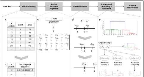
The pipeline of the proposed method, which is named the AliClu, is illustrated in Fig.1. In the first step, the com-plete raw data are pre-processed to obtain the temporal sequences. Then, in the second step, pairwise tempo-ral sequence alignment is performed, and a similarity matrix is obtained. The third step consists of converting the similarity matrix into distances. Agglomerative clus-tering is then performed by using this distance matrix, and finally, the clustering results are validated via a bootstrapping approach. The obtained patient stratifica-tion can be graphically represented to ease the clinical interpretation. Each step of this pipeline is detailed as follows.
Data pre-processing
This pre-processing step creates temporal sequences for each patient from EMRs. Patients’ records are typically available inpanel data format, in which each patient is
spread in different lines, one for each medical appoint-ment, and the columns contain the features of interest measured over time. In this work, we consider that each patient experiences a sequence of events over time. Let A and B be the events of interest for a given patient with the time-distancetbetween them, and aprefix-encoded(PE) sequence for that patient is defined as 0.A,t.B.
In this pre-processing phase, the PE sequences are built for each patient, requiring information about the patient’s ID, the event under study, and the time between two con-secutive events. These features must be taken from the panel data. In the data set, the time may be formatted as a date or just a number in any time unit (e.g., seconds, minutes, or days). Depending on the time format, two types of pre-processing steps are implemented. We refer the interested reader to the Additional file1for further details.
Temporal sequence alignment
After building the prefix-encoded (PE) sequences, it is possible to align all patient pairs using the TNW algo-rithm [1]. The TNW guarantees convergence to the opti-mal alignment for a given scoring scheme, gap penalty
g, and temporal penaltyTp. Notwithstanding, alignments can drastically change depending on the choice of these parameters, and this is the reason why they should be carefully chosen.
The information of the retrieved alignments is summa-rized into anN×N similarity matrixS, where N is the number of patients in the data. In this matrix, the entry value(i,j)gives the alignment score of thei-th andj-th patients. Due to symmetry, onlyN ×(N −1)/2 entries need to be computed.
Distance matrix
Before using the agglomerative clustering algorithm, we need to convert the similarity matrix S, which was obtained in the previous step, into a distance matrixD. To this end, we take the symmetric value of each score and then we shift it by adding the maximum similarity score in matrixS. This shift is made in order to make all scores greater than or equal to zero. In summary, the distance matrix is computed as follows:a= maxi<jSij withi,j = 1,. . .,N and D= −S+a1·1Twith1=
1
.. .
1
∈RN.
Clustering of temporal sequence alignments
Fig. 1The proposed AliClu approach. First, raw data is pre-processed to obtain PE sequences. Then, pairwise sequence alignment is performed and a similarity matrixSis obtained. Next,Sis converted into a distance matrixD. Agglomerative clustering is then performed with this distance matrixD. Validation of the clustering results is accomplished via a bootstrapping approach. In the end, retrieved clusters are analysed by the clinicians
method. Since hierarchical clustering methods do not explicitly set the number of clusters, the AliClu addition-ally provides an automatic bootstrapping-based validation technique proposed by Mucha [17] that selects the best number according to several clustering indices. These indices includeRand[18], theadjusted Rand(AR) [19],
Fowlkes and Mallows(FM) [20],Jaccard, and theadjusted Wallace(AW) [21].
The pseudo-code of the cluster and validation proce-dure is given in Algorithm 1. The inputs of the algorithm are the distance matrixDfor the agglomerative clustering algorithm, the number of bootstrap samplesM, the link-age criterionL, and the minimumKminand the maximum
Kmax numbers of clusters to be analysed. The output is
the statistics of all the clustering indices described above, namely, the medians, means, and variances for all the bootstrap samples, which are calculated for each analysed number of clusters (betweenKminandKmax).
The algorithm begins by performing agglomerative clustering on distance matrixDin Step 1. Then, an outer loop starts in Step 2, corresponding to a bootstrapping procedure. From Steps 3 to 5, a bootstrapped sample is generated, and agglomerative clustering is performed on it. Then, an inner loop computes the clustering indices between the clustering of the original patients and the clustering of the bootstrapped sample (Steps 6-10). In Step 8, the obtained dendrograms Z and Z are cut to
Algorithm 1Agglomerative clustering
1: Perform agglomerative clustering on distance matrix
D, outputing a dendrogramZ.
2: RepeatMtimes:
3: - Bootstrap sample – randomly select 34 patients
from the original data.
4: - Create a new distance matrixDfor the bootstrap
sample.
5: - Perform agglomerative clustering onD with L
which outputs a dendrogramZ.
6: - Letq=Kmin.
7: Whileq≤Kmax:
8: - Cut dendrogramsZandZin order to obtainq
clusters in each.
9: - Compute Rand, AR, FM, Jaccard, and AW between the original and bootstrap partition.
10: - Letq=q+1.
11: Evaluate statistics of the M computations for each
analysedq.
retrieve q clusters (in each), where Kmin ≤ q ≤ Kmax.
After running the outer loopMtimes, the statistics of the clustering indices are computed (Step 11).
the one that yields the higher number of maximum aver-age values over the clustering indices. To corroborate the previous guess, the standard deviation of the clustering indices for eachkcan be taken into account. The choice of
kcan be automatic or semi-automatic. In this latter case, the results composed by dendrograms, the averages and the standard deviations of the obtained clustering indices are given to the user for manual inspection and further selection.
After obtaining the best number of clusters k accord-ing to these criteria, the stability of each individual cluster is then assessed in Algorithm 2, again via the boot-strapping approach [17]. The inputs of this algorithm are the number of clusters k, the clusters themselves {A1,. . .,Ak}, the linkage criterionL, and the number of bootstrapped samplesM. The output is the stability mea-sures of the obtained clusters, which are assessed by the criteria described as follows.
Algorithm 2Cluster stability assessment
1: RepeatMtimes:
2: - Bootstrap sample – randomly select34patients from the original data.
3: - Create a new distance matrixDfor the bootstrap sample. 4: - Perform agglomerative clustering onDwithL, which outputs a
dendrogramZ.
5: - Obtain a collection ofkclusters{B1,. . .,Bk}by cutting the
dendro-gramZ. 6: - Letj=1. 7: Whilej≤k:
8: - Letτj∗=maxi=1,...,kτ(Aj,Bi).
9: - Letγ∗
j =maxi=1,...,kγ (Aj,Bi).
10: - Letη∗
j =maxi=1,...,kη(Aj,Bi).
11: - Letj=j+1.
12: Evaluate statistics of theMcomputations for each analyzed cluster.
The algorithm starts with resampling. For each boot-strapped sample, a dendrogramZis obtained by perform-ing agglomerative clusterperform-ing on the sample (Steps 2-4). Then, a collection of k clusters{B1,. . .,Bk} is obtained by cutting the dendrogram Z (Step 5). From Steps 6 to 11, as proposed by Mucha [17], three different mea-sures are computed for each cluster Aj, 1 ≤ j ≤ k, namely,τj∗(the Jaccard index),γj∗(the recovery rate) and η∗
j (the Dice coefficient). These indices provide a mea-sure of the similarity between cluster Aj and its most similar cluster in{B1,. . .,Bk}. Finally, in Step 12, the sta-bility of the retrieved clusters is assessed by computing the average values ofτj∗,γj∗andη∗j, and by analysing the corresponding standard deviations.
As discussed in [17], it is difficult to set an appropriate threshold that denotes that a cluster is stable. Therefore, we followed the rule of thumb and considered stable clus-ters as the ones that yield high average values (close to one) and low standard deviations forτj∗,γj∗andη∗j.
Algorithm 3 presents the overall proposed method for obtaining clusters from PE sequences. Its inputs are the
raw data, the scoring system SS, the temporal penalty
Tp, and the gap related parameters (gmin,gmaxandgistep) required by the TNW; the number of bootstrapped sam-ples M, for Algorithm 1 and Algorithm 2; the linkage criterion L; and the minimum Kmin and the maximum
Kmaxnumbers of clusters.
Algorithm 3AliClu
1: Pre-process raw data to obtain PE sequences. 2: Letg=gmin.
3: Whileg≤gmax:
4: - Perform pairwise alignment using TNW algorithm with PE sequences,SS,Tpandgas input.
5: - Convert similarity matrixSinto a distance matrixD. 6: - Run Algorithm 1 withD,M,L,Kmin, andKmaxas input.
7: - Letg=g+gistep.
8: Perform consensus decision on the number of clusters given the results from different gapsg.
9: Run Algorithm 2 to assess cluster stability with the bestk clusters
{A1,. . .,Ak},L, and andMas input.
The initial step of the algorithm pre-processes the raw data to produce PE sequences (Step 1). The gap penalty of the TNW algorithm is then set to range fromgminto
gmax at incremental steps of gistep (Step 2 and Step 7). For each value of the gap penalty g, pairwise temporal alignment using the TNW is performed, which outputs a similarity matrixS (Step 4). Then,S is converted into a distance matrixD(Step 5). Clustering is then performed by running Algorithm 1 (Step 6).
When the cycle from Steps 3 to 7 ends, there are several results to explore: one for each of the number of clus-ters (Kmin,. . . ,Kmax) and gap penalties (gmintogmaxwith
gistep). In Step 8, the final number of clusterskis obtained from these results. As stated before, if an automatic proce-dure is chosen, the final number of clusterskretrieved in this step is that which results in the most frequent higher average values for the clustering indices. In this case, the chosen gap penaltygis the one that yields the best aver-age values for the clustering indices for the final number of clusters. In the semi-automatic option, the full results for differentk andg – including the dendrograms, aver-ages and standard deviations of the clustering indices – are provided to the user, which then determines the final number of clusterskand gap parameterg to be further used. In Step 9, the stability of the retrieved clusters is assessed by running Algorithm 2.
The run-time complexity of the TNW isO(n2), and that of agglomerative clustering isO(N3), wherenis the length of the PE sequences andNis the number of patients in the data. Moreover, computing the cluster stability in Algo-rithm 2 for Steps 6–11 takesO(Kmax2 ×N). Therefore, the AliClu algorithm takes
Fig. 2Percentage of biologic drugs taken by Rheumatoid Arthritis (RA) patients. Almost 60% of the patients only had one biologic drug. Patients that have taken more than five biologic drugs are rare; three patients have taken five, two patients have taken six, and other two seven biologic drugs
time, whereG = gmax−gmin+1 gistep
is the number of gaps analysed (gmin to gmax with gistep), M is the number of bootstrapped samples, and K = Kmax − Kmin + 1
is the number of clusters considered (from Kmin to
Kmax).
Results
Synthetic datasets
We first evaluate the AliClu using synthetic datasets, which provides a proof of concept in a controlled sce-nario where the true cluster labels are known a priori and
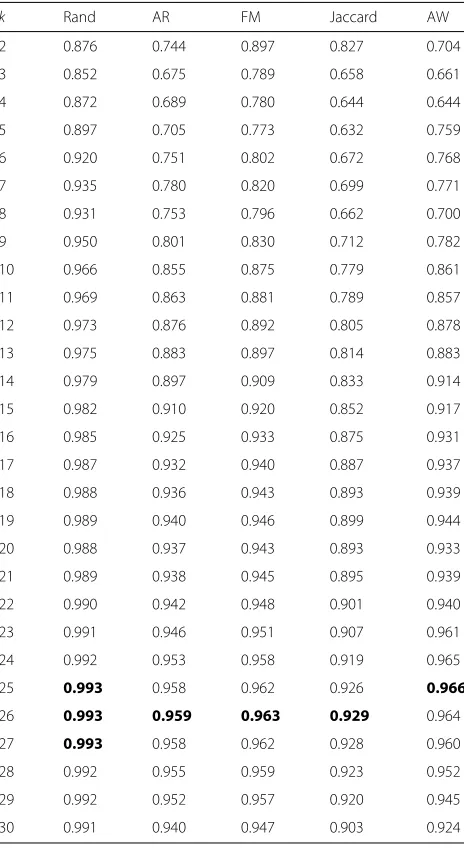
Table 1Average values of five clustering indices for the
dendrogram of Fig.3
k Rand AR FM Jaccard AW
2 0.876 0.744 0.897 0.827 0.704
3 0.852 0.675 0.789 0.658 0.661
4 0.872 0.689 0.780 0.644 0.644
5 0.897 0.705 0.773 0.632 0.759
6 0.920 0.751 0.802 0.672 0.768
7 0.935 0.780 0.820 0.699 0.771
8 0.931 0.753 0.796 0.662 0.700
9 0.950 0.801 0.830 0.712 0.782
10 0.966 0.855 0.875 0.779 0.861
11 0.969 0.863 0.881 0.789 0.857
12 0.973 0.876 0.892 0.805 0.878
13 0.975 0.883 0.897 0.814 0.883
14 0.979 0.897 0.909 0.833 0.914
15 0.982 0.910 0.920 0.852 0.917
16 0.985 0.925 0.933 0.875 0.931
17 0.987 0.932 0.940 0.887 0.937
18 0.988 0.936 0.943 0.893 0.939
19 0.989 0.940 0.946 0.899 0.944
20 0.988 0.937 0.943 0.893 0.933
21 0.989 0.938 0.945 0.895 0.939
22 0.990 0.942 0.948 0.901 0.940
23 0.991 0.946 0.951 0.907 0.961
24 0.992 0.953 0.958 0.919 0.965
25 0.993 0.958 0.962 0.926 0.966
26 0.993 0.959 0.963 0.929 0.964
27 0.993 0.958 0.962 0.928 0.960
28 0.992 0.955 0.959 0.923 0.952
29 0.992 0.952 0.957 0.920 0.945
30 0.991 0.940 0.947 0.903 0.924
makes it easy to determine the merits of the method. The synthetic datasets consisted of temporal sequences gen-erated bycontinuous-time Markov chainsin a variety of parameter settings.
We concluded that the AliClu successfully found the correct clusters in more than 80% of the cases for datasets containing two well-separated clusters. Moreover, the linkage method that produced the best results for the agglomerative clustering was Ward’s method; thus, it was adopted in the remaining experiments. The complete study of the AliClu behaviour on each of the synthetic problems is available in the Additional file1, along with all the details regarding the sequence generation and cluster-ing evaluation.
The Reuma.pt database
We then applied the AliClu to biologic therapy switching forrheumatoid arthritis(RA) patients in a real-life longi-tudinal cohort – the Reuma.pt database [11].
Reuma.pt [11] is a Portuguese nationwide database developed by the Portuguese Society of Rheumatology. It stores the EMRs of rheumatoid patients as struc-tured and narrative data with the goal of monitoring the disease’s progression and assuring treatment effec-tiveness and safety. In this study, we focus on patients withrheumatoid arthritis(RA) being treated with biologic therapies at one centre. The retrieved data include 426 patients diagnosed with RA who followed-up regularly more or less every three to six months, which resulted in a total of 9305 medical appointments.
The RA is an immunomediated inflammatory rheumatic disease that causes pain and swelling in the wrists and small joints of the hands and feet. RA treatments can mitigate these symptoms, prevent joint damage, and provide a better quality of life to the patients. Traditional therapies consist of using conventional disease-modifying antirheumatic drugs
(DMARDs), which are used as a monotherapy or in combinations. When patients fail to respond to conven-tional DMARDs, modern biologic therapies are tried. Unlike conventional DMARDs, biologic ones are made using biotechnology. Biologics are genetically engi-neered to act as natural proteins in the human immune system.
The goal of RA treatment is to induce the disease’s remission by controlling the inflammation. This approach would relieve the symptoms, prevent joint and organ dam-age, improve physical functioning and overall well-being, and reduce long-term complications. It is crucial to iden-tify the most effective RA treatments early in the disease’s progression. In this regard, we used the AliClu to analyse biologic therapy switching, where PE sequences are built by interspersing biologic drugs that are coded as letters and include their durations. The optimized clusters allow for the stratification of RA patients based on their tempo-ral therapy profiles and identification of common features of these groups. Patients starting new biologic therapies can then benefit from these insights.
Clustering of biologic therapy switches
therapies, a patient never goes back to taking the previous biologic drug.
For this particular dataset, the following drugs were as follows: A – etanercept, B – infliximab, C – ritux-imab, D – adalimumab, E – anacinra, F – abatacept, G – tocilizumab, and H – golimumab. These drugs correspond to distinct active therapeutic principles and are prescribed in different stages of the disease.
Having the PE sequences, Algorithm 3 is run with
Kmax = 30, and all other input parameters are set to
their default values. The scoring system is 1 for a match and −1.1 for a mismatch of the drug representation, the temporal penalty isTp = 0.25, and the number of bootstrapped samples is M = 1000. Moreover, in this experiment, the AliClu is used in a semi-automatic man-ner (Step 12 of Algorithm 1 and Step 8 of Algorithm 3 are subject to user input).
We concluded that Ward’s linkage leads to superior results in terms of the clustering indices and clinical infor-mation, and a gap penalty of g = 0.7 and a temporal penalty of Tp = 0.25 correspond to balanced choices with respect to the other input parameters. It is notewor-thy that these choices are data dependent and provide a proof-of-concept of the principle since a full analysis and optimization of the clustering parameters would be out of the scope of the present work.
The running time recorded for this final setting was approximately 1 hour by using a machine with a 2.6 GHz Intel Core i7 processor and 16 GB of 2400 MHz DDR4 memory. This time corresponds to approximately 3.8 seconds for each gap and replicate analysed for the full range of cluster numbers.
Figure 3 shows the dendrogram obtained when using this parameter set, i.e.,g = 0.7 and a temporal penalty ofTp = 0.25. The averages of the five clustering indices obtained with Algorithm 1 are presented in Table1.
Three of the measures, namely, the AR, FM, and Jaccard, indicate the existence of 26 clusters; the AW indicates that
k = 25, and the AR indicates thatk = 25, 26 and 27. In this case, not all averages point to the same number of clustersk; therefore, a more careful and refined analysis is required.
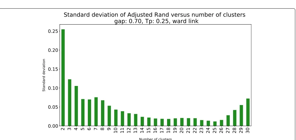
We complemented this analysis with the standard devia-tion of the AR, which is presented in Fig.4. The minimum standard deviation of the AR is achieved for k = 25, which, combined with the information provided in Table1
and Fig.4, leads to the selection of 25 clusters.
The stability of the 25 clusters was then assessed through the medians, averages and standard deviations of η∗,τ∗ andγ∗ (Table2). As expected, the three statistic
values ofη∗are always smaller than those ofτ∗ andγ∗. For some clusters, the medians and averages of the three measures are not as high as is desirable to consider the clusters stable. Moreover, the medians and averages ofτ∗
andγ∗are not the same in all clusters. Notwithstanding, in clusters 20, 21, 22, 23, 24, and 25 (also those with more observations), those values are the same, and they are high enough to be considered stable.
Clusters visualization
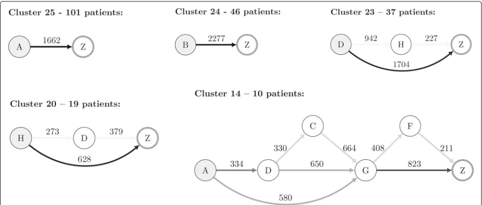
Visualization is an essential task in any clustering pro-cess since it provides an intuitive way to validate clusters. Due to the characteristics of the clustered PE sequences, we propose a graph representation that summarizes the information regarding the sequences that belong to a given cluster. Therein, each node represents a biologic drug symbol (“A” to “H”, and “Z” described above), and each edge represents a therapy switch (from one bio-logic drug to another). A special symbol “Z” marks the end of the sequence, signalling that from that point on there is no information regarding the therapy’s success or failure. The value on an edge is the median of the times between the corresponding drug switches in that cluster.
The colour of an edge represents the transition proba-bility from one biologic drug to another. This probaproba-bility is computed by counting the number of times a switch occurs divided by the total number of transitions in that cluster. A grey scale is used for the edges in this regard. A darker edge means that the switches between the linked biologic drugs frequently occurred in that cluster.
Table 2Stability of the 25 clusters for Ward’s method,g=0.7, andTp=0.25
Cluster Nb. τ∗ η∗ γ∗ τ∗ η∗ γ∗ τ∗ η∗ γ∗
(# patients) median median median average average average std std std
1 (4) 0.475 0.298 0.625 0.475 0.298 0.625 0.389 0.185 0.177
2 (4) 0.750 0.429 0.750 0.750 0.429 0.750 0.000 0.000 0.000
3 (5) 0.083 0.077 0.200 0.083 0.077 0.200 0.000 0.000 0.000
4 (5) 0.400 0.271 0.600 0.400 0.271 0.600 0.283 0.147 0.000
5 (5) 0.275 0.215 0.500 0.275 0.215 0.500 0.035 0.022 0.141
6 (6) 0.833 0.455 0.833 0.833 0.455 0.833 0.000 0.000 0.000
7 (7) 0.741 0.423 0.786 0.741 0.423 0.786 0.164 0.054 0.101
8 (7) 0.307 0.233 0.500 0.307 0.233 0.500 0.080 0.047 0.101
9 (7) 0.643 0.390 0.643 0.643 0.390 0.643 0.101 0.037 0.101
10 (8) 0.688 0.407 0.688 0.688 0.407 0.688 0.088 0.031 0.088
11 (9) 0.542 0.347 0.611 0.542 0.347 0.611 0.177 0.075 0.079
12 (9) 0.389 0.269 0.444 0.389 0.269 0.444 0.236 0.124 0.157
13 (10) 0.352 0.256 0.400 0.352 0.256 0.400 0.145 0.080 0.141
14 (10) 0.489 0.311 0.550 0.489 0.311 0.550 0.337 0.156 0.354
15 (13) 0.513 0.330 0.577 0.513 0.330 0.577 0.254 0.112 0.163
16 (13) 0.472 0.321 0.577 0.472 0.321 0.577 0.039 0.018 0.054
17 (14) 0.571 0.358 0.571 0.571 0.358 0.571 0.202 0.082 0.202
18 (16) 0.719 0.416 0.719 0.719 0.416 0.719 0.133 0.045 0.133
19 (17) 0.309 0.235 0.353 0.309 0.235 0.353 0.084 0.049 0.083
20 (19) 0.716 0.416 0.737 0.716 0.416 0.737 0.119 0.041 0.149
21 (20) 0.791 0.440 0.825 0.791 0.440 0.825 0.154 0.048 0.106
22 (32) 0.696 0.410 0.719 0.696 0.410 0.719 0.056 0.019 0.088
23 (37) 0.791 0.441 0.811 0.791 0.441 0.811 0.104 0.032 0.076
24 (46) 0.728 0.420 0.728 0.728 0.420 0.728 0.108 0.036 0.108
25 (101) 0.777 0.437 0.777 0.777 0.437 0.777 0.007 0.002 0.007
Fig. 5Cluster Visualization. Graph representation of selected clusters based on stability measures and clinical interpretation. Drug codes: A -Etanercept; B - Infliximab; C - Rituximab; D - Adalimumab; E - Anacinra; F - Abatacept; G - Tocilizumab; H - Golimumab. Z - Follow-up/end
the obtained clusters from a medical point of view and highlights the advantages of patient stratification using longitudinal data.
Conclusions
We propose the AliClu, a method that combines tem-poral sequence alignment and agglomerative hierarchical clustering to find groups in longitudinal data containing sequences of symbols and numeric values. The AliClu includes a clustering validation strategy based on boot-strapping and uses several clustering indices, such as the (adjusted) Rand, Fowlkes–Mallows, Jaccard, and adjusted Wallace, to choose the best number of groups to consider for each particular dataset. The stability of the obtained clusters is then assessed through resampling and by using the Jaccard index, the recovery rate, and the Dice indices coefficient. The AliClu can either be run entirely auto-matically or in a semi-automatic way, which requires user input regarding the chosen parameters. The final clus-ters are depicted in graphs where each node represents a symbol, each edge (a state switch) has one number corre-sponding to the median time, and the weight represents the estimated conditional probability of switching.
The AliClu was tested using synthetic data generated with continuous-time Markov chain models, which makes it possible to separate the sequences generated with differ-ent parameters. The AliClu was run using the Portuguese Rheumatic Diseases Register (Reuma.pt), the national database for all the rheumatic patients treated with bio-logic agents. In particular, the rheumatoid arthritis (RA) patients’ therapy information, including the sequence of drugs taken and their durations, was used as the input.
The procedure allowed us to stratify RA patients in a clinically relevant way by creating groups of similar treat-ment profiles. The clusters obtained depict the treattreat-ment switches between different drugs, their median duration times and their probabilities.
The AliClu provides a strategy setting, validation, and visualization procedure for the automatic clustering of temporal sequence data, and it has promising applications for patient stratification using electronic medical record (EMR) data.
Availability and requirements Project name: AliClu
Project home page: https://github.com/sysbiomed/ AliClu
Operating system(s): Platform independent Programming language: Python
Other requirements: Python3 (in Linux or Windows) and Anaconda (in Mac OS)
License: Free
Any restrictions to use by non-academics: None
Supplementary information
Supplementary informationaccompanies this paper at https://doi.org/10.1186/s12911-019-1013-7.
Additional file 1: Supplementary Information
Abbreviations
Acknowledgments
We acknowledge all Reuma.pt contributors.
Authors’ contributions
KR implemented the algorithms, performed the computational experiments and wrote the first draft of the manuscript (all authors made the required updates). HC provided the data, clinical insights and interpretation. AMC and SV conceived the study, supervised the research, generated the final results and manuscript. All authors contributed to the final draft, read and approved the final version of the manuscript.
Funding
The authors acknowledge funding the Portuguese Foundation for Science and Technology (Fundação para a Ciência e a Tecnologia - FCT) under contracts INESC-ID (UID/CEC/50021/2019) and IT (UID/EEA/50008/2019), projects PREDICT (PTDC/CCI-CIF/29877/2017), PERSEIDS
(PTDC/EMS-SIS/0642/2014) and NEUROCLINOMICS2 (PTDC/EEI-SII/1937/2014). The funders had no role in the design of the study, collection, analysis and interpretation of data, or writing the manuscript.
Availability of data and material
AliClu is available athttps://github.com/sysbiomed/AliClu. Data from Reuma.pt are not publicly available. Synthetic data is provided along with AliClu to ease its use.
Ethics approval and consent to participate
Reuma.pt was approved by the National Data Protection Board (Comissão Nacional de Proteção de Dados – CNPD, Portugal) and by the Ethics Committee of Centro Hospitalar Lisboa Norte (CHLN) - Hospital de Santa Maria (HSM), Lisbon, Portugal. Patients signed Reuma.pt’s informed and written consent.
Consent for publication Not applicable.
Competing interests
SV is member of the Editorial Board of BMC Bioinformatics. KR, HC, and AMC declare that they have no competing interests.
Author details
1Instituto de Telecomunicações, Instituto Superior Técnico, Universidade de
Lisboa, Avenida Rovisco Pais, 1 - Torre Norte Piso 10., 1049-001 Lisboa, Portugal.2CEDOC, EpiDoC Unit, NOVA Medical School, National School of
Public Health, Universidade NOVA de Lisboa, Rua do Instituto Bacteriológico, n◦5 Lab 2.9., 1150-082 Lisboa, Portugal.3INESC-ID, Instituto Superior Técnico,
Universidade de Lisboa, Rua Alves Redol 9, 1000-029 Lisboa, Portugal.
Received: 24 June 2019 Accepted: 19 December 2019
References
1. Syed H, Das AK. Temporal Needleman-Wunsch. In: 2015 IEEE International Conference on Data Science and Advanced Analytics (DSAA). IEEE; 2015.https://doi.org/10.1109/dsaa.2015.7344785. 2. Needleman SB, Wunsch CD. A General Method Applicable to the Search
for Similarities in the Amino Acid Sequence of Two Proteins. J Mol Biol. 1970;48:443–53.
3. Sakoe H, Chiba S. Dynamic programming algorithm optimization for spoken word recognition. IEEE Trans Acoust Speech Sig Process. 1978;26: 43–9.
4. Zhou F, la Torre FD. Canonical time warping for alignment of human behavior. In: Advances in Neural Information Processing Systems 22: 23rd Annual Conference on Neural Information Processing Systems 2009. Vancouver: Curran Associates, Inc.; 2009. p. 2286–94.
5. Kulkarni K, Evangelidis G, Cech J, Horaud R. Continuous action recognition based on sequence alignment. Int J Comput Vis. 2015;112(1): 90–114.https://doi.org/10.1007/s11263-014-0758-9.
6. Fischer B, Roth V, Buhmann JM. Time-series alignment by non-negative multiple generalized canonical correlation analysis. BMC Bioinformatics. 2007;8(10):4.
7. Sievers F, Wilm A, Dineen D, Gibson TJ, Karplus K, Li W, Lopez R, McWilliam H, Remmert M, Söding J, Thompson JD, Higgins DG. Fast, scalable generation of high-quality protein multiple sequence alignments using clustal omega. Mol Syst Biol. 2011;7(1):539. 8. Katoh K, Standley DM. Mafft multiple sequence alignment software
version 7: Improvements in performance and usability. Mol Biol Evol. 2013;30(4):772–80.
9. Edgar RC. Muscle: multiple sequence alignment with high accuracy and high throughput. Nucleic Acids Res. 2004;32(5):1792–7.
10. Eddy SR. Profile hidden Markov models,. Bioinformatics. 1998;14(9): 755–63.https://doi.org/10.1093/bioinformatics/14.9.755.
11. Canhão H, Faustino A, Martins F, et al. Reuma.pt - The Rheumatic Diseases Portuguese Register. Acta Reumatologica Portuguesa. 2011;36(1):45–56. 12. Docampo E., Collado A., Escaramís G, Carbonell J, Rivera J, Vidal J,
Alegre J, Rabionet R, Estivill X. Cluster analysis of clinical data identifies fibromyalgia subgroups. PLOS ONE. 2013;8(9):1–7.https://doi.org/10. 1371/journal.pone.0074873.
13. Garg L, McClean S, Meenan BJ, Millard P. Phase-type survival trees and mixed distribution survival trees for clustering patients’ hospital length of stay. Informatica. 2011;22(1):57–72.
14. Axén I, Bodin L., Bergström G, Halasz L, Lange F, Lövgren PW, Rosenbaum A, Leboeuf-Yde C, Jensen I. Clustering patients on the basis of their individual course of low back pain over a six month period. BMC Musculoskelet Disord. 2011;12(1):99. https://doi.org/10.1186/1471-2474-12-99.
15. De la Cruz-Mesía R, Quintana FA, Marshall G. Model-based clustering for longitudinal data. Comput Stat Data Anal. 2008;52(3):1441–57.https:// doi.org/10.1016/j.csda.2007.04.005.
16. Saxena A, Prasad M, Gupta A, Bharill N, Patel OP, Tiwari A, Er MJ, Ding W, Lin C-T. A review of clustering techniques and developments. Neurocomputing. 2017;267:664–81.
17. Mucha H-J. Advances in Data Analysis. In: Decker R, Lenz H-J, editors. Berlin, Heidelberg: Springer; 2007. p. 115–122.
18. M. Rand W. Objective criteria for the evaluation of clustering methods. J Am Stat Assoc. 1971;66:846–50.
19. Hubert L, Arabie P. Comparing partitions. J Classif. 1985;2(1):193–218. 20. B. Fowlkes E, Mallows C. A method for comparing two hierachical
clusterings. J Am Stat Assoc. 1983;78:553–69.
21. Wallace DL. A method for comparing two hierachical clusterings: Comment. J Am Stat Assoc. 1983;78:569–76.
Publisher’s Note