http://www.sciencepublishinggroup.com/j/ajsea doi: 10.11648/j.ajsea.s.2016050301.16
ISSN: 2327-2473 (Print); ISSN: 2327-249X (Online)
Optimization Algorithms Incorporated Fuzzy Q-Learning for
Solving Mobile Robot Control Problems
Sima Saeed, Aliakbar Niknafs
Department of Computer Engineering, Faculty of Engineering, Shahid Bahonar University of Kerman, Kerman, Iran
Email address:
[email protected] (S. Saeed), [email protected] (A. Niknafs)
To cite this article:
Sima Saeed, Aliakbar Niknafs. Optimization Algorithms Incorporated Fuzzy Q-Learning for Solving Mobile Robot Control Problems.
American Journal of Software Engineering and Applications. Special Issue: Advances in Computer Science and Information Technology in Developing Countries. Vol. 5, No. 3-1, 2016, pp. 25-29. doi: 10.11648/j.ajsea.s.2016050301.16
Received: September 14, 2016; Accepted: September 23, 2016; Published: August 21, 2017
Abstract:
Designing the fuzzy controllers by using evolutionary algorithms and reinforcement learning is an important subject to control the robots. In the present article, some methods to solve reinforcement fuzzy control problems are studied. All these methods have been established by combining Fuzzy-Q Learning with an optimization algorithm. These algorithms include the Ant colony, Bee Colony and Artificial Bee Colony optimization algorithms. Comparing these algorithms on solving Track Backer-Upper problem –a reinforcement fuzzy control problem– shows that Artificial Bee Colony Optimization algorithm has the best efficiency in combining with fuzzy- Q Learning.Keywords:
Mobile Robot, Fuzzy-Qlearning, Ant Colony Optimization-Fuzzy Q Learning, Bee Colony Optimization-Fuzzy-Q Learning, Artificial Bee Colony-Fuzzy Q Learning1. Introduction
In the recent years, applying fuzzy systems in the various places has been an important subject to investigate. In general, the implementation of a fuzzy system depends on the fuzzy system rules and also on input/output membership functions. However, obtaining these information from the experts' previous knowledge source is not always easy and possible. In order to overcome this problem, many researchers have attempted to find some automatic methods for designing the fuzzy system. These methods are divided into two classes: monitoring learning- based schema and reinforcement learning – based schema. For these problems, reinforcement learning is superior to monitoring learning. In the reinforcement learning, factor obtains a critic from the environment which is referred to reinforcement and indeed is a kind of reward or punishment. In fact, the factor is not told what to do but instead of the factor must study the different actions and detect which one will have the most awards. One of the most famous methods in this kind of learning is Q learning. Q learning method is usually used in the environments with discontinuous states and performances. The idea of Fuzzy- Q learning which the developed kind of ordinary Q learning is has been developed to work on the
environments with continuous states and performances. In the Fuzzy-Q learning, the result part of every rule is independently and locally selected by its Q indices and reselected in every time stage. The best combination of result part in every rule is not considered during selection. To select the best combination of result part, the optimization algorithms can be used. In the present paper, the structure related to some of these methods including Ant Colony Optimization-Fuzzy Qlearning (ACO-FQ), Bee Colony Optimization-Fuzzy Qlearning (BCO-FQ) and Artificial Bee Colony-Fuzzy Qlearning (ABC-FQ) are explained. In the last part of this article, these three methods on solving Track-Backer Upper problem are described.
2. Background and Preliminaries
Q-value t , . The output of a Q-function, called the Q-value, is updated by
t , ← t , . 1
∗ t 1 t , (1)
Where t 1 is the state that is obtained from t after the execution of , 1 is the reinforcement from the environment, is the learning rate, is a discount factor, and ∗ t 1 is the best estimated Q-value that the agent thinks it can get at state t 1 , which is defined by
∗ t 1 max
∈ ! t , " (2)
Where # t 1 is the set of possible actions in state
t 1 . The learning rate , 0 &α ' 1 , is a constant
step-size parameter that determines the updating speed of the Q-function. The discount factor ,0 ' ' 1, determines the present value of future rewards [1-4].
3. Optimization Algorithms Incorporated
with Fuzzy Q-Learning
3.1. Ant Colony Optimization-Fuzzy Q Learning (ACO-FQ)
The fuzzy inference system designed by ACO-FQ is composed of singleton type fuzzy if-then rules with the following form:
(): +, ! +- .)! /0, . . . , /0 1 +- .)1 23/ 4 +- 5! 6+ 2 7)!
8 59 6+ 2 7)9 . . . 8 5: 6+ 2 7):
Where ! , . . . , 1 are the input variables, is the output action variable, .)!, . . . , .)1 in are fuzzy sets, and
) is a recommend action consequent can be directly chosen from the candidate actions # ; 5!, . . , 51< by ACO and fuzzy Q-learning. Consider L rules in a fuzzy inference system, where a weighted average defuzzification method is used. For calculating the output of the system, we have to decide one from a total of f => combinations of consequent parts. This problem could be solved by ACO-FQ. In this method, a combination of consequent actions is considered as the tour of an ant. It is selected from every rule. To enable the ant colony to exploit the q-value information, the q-value is used to replace the heuristic value in the transition probability function in:
?)@ ABCD EBCF G
∑JIKLABID EBIF G + 1, … , N, O 1, … , = (3)
The influence weighting of P and q is controlled by parameter Q. Q-value is given by
R , 4 R ∑XBKLSB R T .UBV̂
∑XBKLSB R T (4)
Y) R is the firing strength and 4 R is the value of the final system action. The update of the q-values in each rule is as
7)@ 1 7)@ Z. ∆7)@ (5)
Where ε is a learning rate.
∆7)@ ∆ . SB R T
∑XBKLSB R T . 3)@ (6)
3)@ represents eligibility trace [5]. The pheromone level
P)@ is updated by the following equation:
P)@ \ P)@ \ ∆P)@ \ (7)
∆P)@ \ ]^̂. _ +, +, O ∈ 23 / 85 0 23 8 23 6+-3 (8)
Where ^̂ denotes the learning rate for local updating speed of τ. F is fitness value in ACO and stores total number of time steps until failure. In the global update rule, the ant that achieves the maximum number of time steps F is found. Then, the pheromone levels are updated with:
∆P)@ \ ]^. _ +, +, O ∈ + 3 +8/ "3- 850 23 8 23 6+-3 (9)
Where ^ denotes the learning rate for global updating speed of P. Fig. 1 shows ACO-FQ algorithm [5].
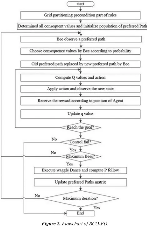
3.2. Bee Colony Optimization-Fuzzy-Q Learning (BCO-FQ)
In this algorithm to implementation its BCO we have two separate sets: (1) Preferred Path Set, (2) Consequences set. Preferred path set includes a combination of Consequences set and its size is equal to the number of rules [6-7]. At the beginning of the algorithm, we randomly provide a population in size of Max Bee Colony from these preferred path sets. Indeed, this set is a guide for the bee. Fig. 2 shows the trend of BCO-FQ algorithm working.
Figure 2. Flowchart of BCO-FQ.
3.3. Artificial Bee Colony-Fuzzy Q Learning (ABC-FQ)
Overview of ABC-Fuzzy Q learning algorithm is shown in Fig. 3. This algorithm includes three main phases: employed, onlooker and scout bees [8-9]. The algorithm will be finished when the answer is achieved in each of these phases. In ABS-FQ algorithm, N food sources are considered and each food source shows the values of L result rules in a fuzzy system !~ > . Q-Value indicates the nectar amount for each food source 7) . The more the Q-Value of a food source shows that this food source generates a stronger fuzzy system to control the agent [10]. The fuzzy system is considered as follows:
+, ? 3^8/0+ +8/ ? 23/ ^8/-3753/^3
+-_880- 1 !!, … , >! 6+ 2 7!
8 _880- 2 !9, … ,
>9 6+ 2 79
….
8 _880- = !:, … , >: 6+ 2 7:
Whenever a food source of _880- +̂ is selected with 7+̂, a fuzzy system is performed and this system is applied to environment.
Figure 3. Flowchart of ABC-FQ [10].
4. Simulation and Comparison
For comparing the results of proposed method with results of other methods such as ABC-FQ, ACO-FQ and BCO-FQ, the simulation of Truck Backer- Upper has been considered. The objective of this simulation is that a truck moves back automatically and stops in a given location.
In order to control this automobile, we consider 3 inputs of x, y and θ, and one output of α, as illustrated in part 2. In the modeling, it has been assumed that there is enough clearance between truck and loading dock, and thus the y component is not considered as the input [5]. The machine is controlled by computer modeling as follows: (10-12)
1 cos e sin sin e (10)
h 1 h sin e sin cos e (11)
Figure 4. Simulation truck and loading station.
Range of the values for the inputs is e 90°, 270° and
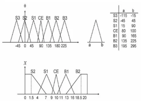
0, 25 , and range of values for the output is 40°, 40°. The truck length is considered to be b = 4. The antecedent part of the rules of fuzzy control is classified by grid type, and 7 fuzzy sets for the input θ and 5 fuzzy sets for the input x are considered according to the Fig 5.
Figure 5. Fuzzy membership functions for the Truck Backer-Upper.
In this mode we have 7 t 5 35 fuzzy rules. The result
part of the rules that are the values, are selected from the set
# 40, . . , 5, 0, 5, . . , 40 ; this selection, and also regulation of α values is performed by algorithms.
The results of BCO-FQ method demonstrate that the machine can find the target after passing helically through the stages in all implementations, however in some cases the time for reaching the target becomes longer but the number of failures of the machine to reach the target is zero.
This case demonstrates the reliability of the proposed method. Table 1.
Table 1. The results of BCO-FQ method.
Method Average
trials
Number of Failure runs
Average CPU Time (sec)
BCO-FQ 632 0 60
Table 2 shows a comparison of efficiency between two methods to solve Truck Backer – Upper problem. As you can see, ABC-FQ method has a better performance than ACO-FQ one.
Table 2. Comparative evaluation of methods.
Method ACO-FQ ABC-FQ
Average trials 365 87
Standard deviation 95 91
Worst (trial Number) 559 393
Number of Failure runs 0 0
Average CPU Time (sec) 10.1 10
Fig. 6 show the results of ABC-FQ method from different starting points. We started this algorithm from 3 different locations, and considered the final location of truck placement (target) by e∈ [80°, 100°] and x∈ [9, 11]. The above mentioned locations are , e = (3, 135°), , e = 12, 45° /0 , e 18, 30° .
Figure 6. Trajectory of the truck, (a). location = , e 3, 135° – (b). Location= , e 12, 45°–(c) Location= , e 18, 30°.
5. Conclusions and Future Work
Consequently, one can conclude that every three proposed methods are of acceptable advantages on solving this problem. The third method has the best quality than the other methods. In order to increase the quality of algorithms, it is proposed that the following cases will be considered in the future research:
-Transforming the fuzzy rules in the precondition part from static state into dynamic state in all algorithms of this article.
-Changing the evolutionary algorithm in combining with
Fuzzy-Q learning algorithm for more optimization.
-Changing in the fuzzy membership functions and studying its influences on reinforcement learning for example establishing the continuous membership functions to give awards to the factor in all algorithms.
References
[1] H. R̒. Berenji, “Fuzzy Q-learning for generalization of reinforcement,” IEEE Int. Conf. Fuzzy Syst, 1996.
[2] P. Y. Glorennec, “Fuzzy Q-learning and dynamic fuzzy Q-learning,” IEEE Int. Conf. Fuzzy Syst., Orlando, 1994. [3] P. Y. Glorennec, L. Jouffe, “Fuzzy Q-learning,” IEEE Int. Conf.
Fuzzy Syst, 1997.
[4] L. Jouffe, “Fuzzy, inference system learning by reinforcement methods̕,” IEEE Trans. Syst., Man, Cybern. C, Appl. Rev., Vol. 28 (3), pp. 338–355, 1998.
[5] C. F. Juang, “Ant Colony Optimization Incorporated With Fuzzy Q-Learning for Reinforcement Fuzzy Control,” IEEE Transactions on systems, man, and cybernetics—part a: systems and humans, Vol. 39, May 2009.
[6] L. P. Wong, M. Yoke Hean Low, C. S. Chong, “A Bee Colony Optimization Algorithm for Traveling Salesman Problem,” Second Asia International Conference on Modelling & Simulation, IEEE, 2008.
[7] L. P. Wong, Y. H. Malcolm Low, C. S. Chong, “Bee Colony Optimization with Local Search for Traveling Salesman Problem,” 2008.
[8] M. Servet Kiran, H. Iscan, M. Gounduz, “The analysis of discrete artificial bee colony algorithm with neighborhood operator on traveling salesman problem,” Neural Comput and Applic, 2013.
[9] W. li. Xiang, M. Qing An, “An efficient and robust artificial bee colony algorithm for numerical optimization,” Computers and Operations Research, pp. 1256–1265, 2013.