New algorithm for biological objects' shape evaluation and data reduction

13

Volume LVIII 1 Number 1, 2010

NEW ALGORITHM FOR BIOLOGICAL OBJECTS’

SHAPE EVALUATION AND DATA REDUCTION

S. Bartoň, L. Severa, J. Buchar

Received: September 2, 2009

Abstract

BARTOŇ, S., SEVERA, L. BUCHAR, J.: New algorithm for biological objects’ shape evaluation and data reduc-tion. Acta univ. agric. et silvic. Mendel. Brun., 2010, LVIII, No. 1, pp. 13–20

The paper presents the so ware procedure (using MAPLE 11) intended for considerable reduction of digital image data set to more easily treatable extent. The example with image of peach stone is pre-sented. Peach stone, displayed on the digital photo, was represented as a polygon described by the co-ordinates of the pixels creating its perimeter. The photos taken in high resolution (and corresponding data sets) contain coordinates of thousands of pixels – polygon’s vertexes. Presented approach substi-tutes this polygon by the new one, where smaller number of vertexes is used. The task is solved by use of adapted least squares method. The presented algorithm enables reduction of number of vertexes to 10 % of its original extent with acceptable accuracy +/− one pixel (distance between initial and fi nal polygon). The procedure can be used for processing of similar types of 2D images and acceleration of following computations.

image processing, data reduction, least square method

The acquisition and analysis of the visual informa-tion represents powerful tool for interpretainforma-tion of large range of input data. The origin of computer vi-sion is intimately intertwined with computer history, having been motivated by a wide spectrum of im-portant applications such as robotics, biology, medi-cine, industry and physics, but also agricultural and food sciences in last decades. Among all diff erent as-pects underlying visual information, the shape of the objects certainly plays a special role. The multi-disciplinarity of image analysis, with respect to both techniques and applications, has motivated a rich and impressive set of information resources repre-sented e.g. by book Costa and Cesar (2009).

Precise and correct image processing enables solv-ing problems of multidisciplinary nature, complet-ing images and objects in terms of features (implycomplet-ing several distinct objects to be mapped into the same representation), pattern recognition used for seg-menting an image into its constituent parts, proper validation of algorithms, and/or improving the rela-tion between continuous and discrete approaches.

In fact “computer vision” (or generally image cessing) o en requires, sometimes real time, pro-cessing of a very large and heterogeneous data sets (including shape, spatial orientation, color,

14 S. Bartoň, L. Severa, J. Buchar

reconstructing the original data points in the data set. This method was successfully used in number of works – see e.g. Vidal et al. (2005), Iglesias et al. (2007), Havlíček et al. (2008). There are alternative approaches such as LDA (Linear Discriminant Anal-ysis) – see e.g. Wang et al. (2004) or PFA (Principal Factor Analysis) – see e.g. Ballester et al. (2005).

This paper presents completely diff erent ap-proach, where input image data are signifi cantly re-duced (to 10 % of original extent) by means of MA-PLE 11 algorithm without loss of precision. Example with peach stone is presented. Reduced data sets can be consequently used for faster processing and/or further utilization. MAPLE so ware environment have been successfully used for determination of agricultural products shape (Bartoň, 2000; Bartoň, 2007; Bartoň, 2008).

MATERIAL AND METHODS

Digital photo

A sample digital photo of peach stone of Red Heaven variety (harvested in July 2008 in region of Southern Moravia) has been used. But any similar object of natural of artifi cial origin could have been used. The photo has been taken by digital camera Olympus SP–55OUZ with resolution of 7.1 Mpixels, see Fig. 1.

Processing so ware

A so ware MAPLE 11, classic has been used to perform all presented calculations.

Computing procedure

The best line

Let us assume polygon given by the list of N points with coordinates [[X1, Y1], …, [Xi, Yi], …, [XN, YN]].

Let us select sublist of vertexes N1 … N2, 1 <= N1 < N2 <= N, N2−N1>= 2. The task is to fi nd parameters of common line p1 which will minimize

N2 ∑ di

2

i=N1 , where

di = length of the line segment between ith and p_ith

point. The point is the intersection of the line per-pendicular to the line p1 going through ith point with

the line p1.

Lists of lines and corresponding points A er defi nition of best line, the procedure can continue in computing of best line for remaining points from the list of the vertexes and smoothing the polygon.

Estimating of accuracy

A er polygon approximation it is possible to com-pute distances d_i for input polygon vertexes using corresponding line segments. It is possible to com-pute their average values and variance. These values may be used to determine accuracy of approxima-tion.

Maple procedure

The complete Maple procedure for presented ap-proach can be seen in the fi rst author’s personal web pages: user.mendelu.cz/barton.

RESULTS AND DISCUSSION

The best line

The best form of the line p1, corresponding to the above mentioned problem is p1: = (x−Qx) sin(φ) + (Qy−y) cos(φ) = 0, where [Qx, Qy] are coordinates of the point lying on this line and φ is its direction an-gle, see Fig. 2.

In this case the coordinates of the p_ith point are as follows:

Xpi = (−Qx cos(φ) − sin(φ) Qy + sin(φ) Yi + Xi cos(φ))

cos(φ) + Qx

and

Ypi = (−Qx cos(φ) − sin(φ) Qy + sin(φ) Yi + Xi cos(φ))

sin(φ) + Qy. (1)

The square of the distance from the line p1 is di

2 ₌ (X_i−Xp_i)2 _{+ (Y}

i−Ypi)

2_{, where Xp}

i and Ypi are defi ned

by the equation (1). The sum of the squares of the distances di for all N points is

N2 ∑ di

2 _{= SoS}

i=N1 , SoS = −2cos(φ) sin(φ) (QyQx (N2 − N1 + 1) + ∑2 − Qy

∑3 − Qy ∑4) + ((N2 −N1 + 1) Qx2_{− 2Qx ∑}

3 + ∑1) sin(φ) 2 + ((N2 −N1 + 1) Qy2_{− 2Qy ∑}

4 + ∑5) cos(φ)2, (2) where

N2 N2 N2 N2 N2 ∑1 = ∑ Xi

2_{, ∑}

2 = ∑ Yi Xi, ∑3 = ∑ Xi, ∑4 = ∑ Yi, ∑5 = ∑ Yi

2

i=N1 i=N1 i=N1 i=N1 i=N1 _. These substitutions accelerate computation of

N2 ∑ di

2

i=N1 , because it is faster to calculate all sums only ones and to substitute obtained results instead of computing each sum as indicated in (2) or in the fol-lowing expressions. The condition for the global minimum of SoS(Qx, Qy, φ) is ⎯⎯∂ SoS = 0

∂Qx ,

∂

⎯⎯SoS = 0

∂Qy and

∂

⎯⎯SoS = 0

∂Qφ . First and second

equa-tion consequently yields in ∑3

Qx = ⎯⎯⎯⎯⎯

N2−N1 + 1, ∑4

Qy = ⎯⎯⎯⎯⎯

N2−N1 + 1. If these values are substituted into the third equation, the result has a following form:

S2 sin(φ) 2 _{+ S}

1 cos(φ)sin(φ) + S3 cos(φ) 2 _{= 0,} where below listed substitutions (3)

S1 = 2∑4 2_{− 2∑}

1N1 + 2∑1− 2∑5− 2∑5N2 + 2∑5N1− 2∑3 2 ₊ 2∑1N2,

S2 = −2∑4∑3 + 2∑2N2− 2∑2N1 + 2∑2,

S3 = 2∑2N1− 2∑2− 2∑2N2 + 2∑4∑3

simplify equation (3) and its solution for φ. Equation (3) has two roots:

⎛ S1

√

2S3⎞

φ1 = arctan ⎜_⎝− ⎯ + ⎯⎯⎯⎯⎯⎟ 2 2S2 ⎠

and

⎛S1

√

2S3⎞

φ2 = arctan ⎜_⎝⎯ + ⎯⎯⎯⎯⎯⎟ 2 2S2 ⎠

. (4) The fi rst root leads to the global minimum of the SoS, the second one to the global maximum. Therefore it is possible to continue with φ = φ1. Fol-lowing substitution

S2

cos(φ) = ⎯⎯⎯⎯⎯⎯⎯⎯⎯⎯⎯⎯⎯⎯⎯

√

√

2S3)

√

√

12 + S1

√

(5) will simplify computations of (4). In special cases, when line p1 is parallel with x or y axis S2 = 0, this substitution converts into cos(φ) = 0, sin(φ) = 1 or cos(φ) = 0, sin(φ) = 0. In these cases, proper values of cos(φ) and sin(φ) must be found, to obtain smaller value of SoS.

Lists of lines and corresponding points The best line for the fi rst three points from the list of vertexes can be computed as follows. Let us assume N1=1 and N2=3 for this particular case. The best line p1 can be foundfor each point with consequent computing of corresponding square of the distance d_i and fi nding the maximum of dis-tances Dist = max([dN1, …, di, …, dN2]. If the value is

16 S. Bartoň, L. Severa, J. Buchar

ing values of Qx, Qy, cos(φ), sin(φ) describing the best line for the vertexes N1 … N2, and Dist can be stored into the lists. The highest N2 satisfying condition

Dist < kL can be determined from these lists, where

k is the correction value depending on smoothness of the polygon. If the polygon is smooth k→ 0.5, for non-smooth polygons k→ 0.2. It is possible to use the value of k ~ 0.5, but it must be considered that value Dist is function of N2 and if it ones exceeds k L, it may be again lower for higher value of N2. This ap-proach leads to higher number of fi nal polygon ver-texes. In this case the data reduction will not be so eff ective. The reason, why the value k = 1 cannot be used will be discussed later.

As a next step, the points [Xp_N1, Yp_N1], [Xp_N2, Yp_N2]

must be recorded into the list LXY, ordinary num-bers of the border points N2 are recorded into list LN2, and value N1 put equal to N2, (N1 = N2). The whole process can be repeated with the sub-sequent vertexes from the list of polygon vertexes. The procedure is repeated until N2 < N. Finally, the both lists will contain n elements. The list LXY

can be displayed as a list of separate line segments approximating initial polygon. The ordinary num-bers of vertexes of the input polygon corresponding to the i-th line can be picked from the list LN2 as se-ries if integer numbers from LN22i−1 to LN22i. These

lists contain information about line segment – best line and input polygon vertexes corresponding to the line segment. But the line segments are not con-nected one with each other – see Fig. 3. The best line segments are displayed as a red-dashed line, input polygon vertexes are displayed as red crosses and polygon vertexes with ordinary numbers N2 are blue-circled. These points correspond to endpoints of the best line segments.

The endpoint of one line segment [Xp_N2, Yp_N2] and

initial point of the subsequent line segment [Xp_N1,

Yp_N1] correspond to the same vertex of the input

polygon. These points are very close, but not iden-tical, because they correspond to the diff erent line segments. The points are displayed in Fig. 3 as blue boxes – end points of the best line segments. These couples of points can be substituted by their mid-points and they are displayed as green diamonds [Xc, Yc] = 5([XpN2, YpN2] + [XpN1, YpN1] in Fig. 3. As a

re-sult, continuous curve is obtained, displayed as black line segments, creating polygon with reduced number of vertexes approximating input polygon. Center points will be recorded in a new list LC. Be-cause new polygon vertex [Xc, Yc] is a midpoint

cor-responding to the projection of the same vertex of the initial polygon to diff erent best lines, this point does not lay on these best lines, but it is close to both of them and the new line segments do not corre-spond to the preceding line segments – best lines. Therefore it is necessary to put k<1. As k→ 0, these line segments are shorter, the number of vertexes of the fi nal polygon increases, but accuracy of the ap-proximation is better. Diff erent scale for x and y axis is used for better overview of Fig. 3. Thus expected right angles are displayed as distorted.

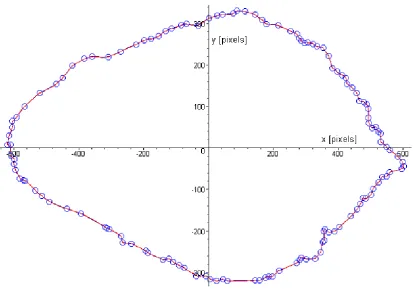
The result can be displayed graphically, see Fig. 4. The fi gure displays peach stone perimeter described by 3866 red points. Corresponding polygon is substi-tuted by polygon with 109 vertexes with predefi ned accuracy of 5 pixels. Approximating polygon is dis-played by blue line and its vertexes are indicated by blue circles. Since the diff erence between blue and red line is smaller then line thickness itself, the blue line is not visible. It can be seen that with data reduc-tion 1:35, the accuracy is satisfying.

Estimating of the accuracy

The most eff ective method is to compute absolute value d_i and argument φ_i of the vector v_i = [X_i−X_pi,

Yi−Ypi], see Fig. 2, which can be used for the

ment is defi ned by its endpoints, [X_c1, Y_c1] and [X_c2,

Yc2], see previous section, the distance di and

orien-tation φi can be computed using very simple

expres-sions:

(X_c2−X_c1) Y_i− (Y_c2−Y_c1) X_i + X_c1 Y_c2 −X_c2 Y_c1 di = ⎯⎯⎯⎯⎯⎯⎯⎯⎯⎯⎯⎯⎯⎯⎯⎯⎯⎯⎯

_√

c2 2_−X

c1) 2 _{+ (Y}

c2−Yc1)

2 ,

⎛ Y_c1−Y_c2 ⎞ φi = arctan ⎜_⎝⎯⎯⎯⎯_X ⎟ c2−Xc1⎠ ,

where (6)

Xc2 = LC2j−1, 1, Yc2 = LC2j−1, 2, Xc1 = LC2j, 1, Yc1 = LC2j, 2,

LN2j<= i <= LN2j+1 and 1<= j <= n.

This approach enables to display accuracy in po-lar coordinates. For the peach stone presented in Fig. 4, the corresponding accuracy is visualized in Fig. 5. As can be seen, the real accuracy is +/− 2 pix-els only. It means that the worst accuracy achieved is about 0.3 % of the object size and the average accu-racy indicated by the thick blue line is +/− 0.7 pixels, approximately 0.1%. Variances of the accuracy are displayed as the thin blue lines.

It is possible to plot vertexes of the input polygon and the resulting polygon. The example with dis-tances di magnifi ed 25-times is shown in Fig. 6.

It is possible to complete the algorithm by weight list – signifi cance of individual points, W. The weight list is intended pro data processing in the so wares directly computing optimum regression function.

The relations can be determined as a mean of length value of both segments trajecting through the points. The relation has a following form:

√

2 _{+ (Y}

c_i−1−Yc_i)

2 ₊

_√

c_i+1−Xc_i)

2 _{+ (Y}

c_i+1−Yc_i)

Wi = ⎯⎯⎯⎯⎯⎯⎯⎯⎯⎯⎯⎯⎯⎯⎯⎯⎯⎯⎯⎯⎯₂ .

(7) The diff erence between regression function with and/or without including of weights is displayed in Fig. 7. The red line represents the function approx-imating the stone’s shape in polar coordinates with coordinate origin in [129.58, 46.647],

Red = 388.90 − 92.140cos(f) − 56.561sin(f) + 102.11cos(2. f)

+ 2.1903sin(2. f) − 37.708cos(3. f) − 15.099sin(3. f) + 48.019cos(4. f) − 0.045109sin(4. f) − 20.729cos(5. f) − 12.624sin(5. f) + 17.420cos(6. f) − 3.9376sin(6. f) − 9.1169cos(7. f) − 9.8685sin(7. f) + 8.3158cos(8. f) − 2.7700sin(8. f) − 9.0515cos(9. f) − 6.4355sin(9. f) (8)

The blue line represents the regression function including weights. The coordinates origin is situated in [1.071, 50.786].

Blue = 394.34 + 6.5714 cos(f) − 61.163 sin(f) + 109.42 cos(2. f)

18 S. Bartoň, L. Severa, J. Buchar

SUMMARY

Extensive image fi les or series of images are to be o en processed and such procedures can represent demanding task for hardware as well as so ware environment. Partial data reduction with maintain-ing the original information and achievement of maximum accuracy is thus eff ective and useful tool for further computations or generally image data processing. This paper introduces the so ware ap-proach of reducing the large volume of digital image data to 3 % of its original extent. MAPLE 11 clas-sic was used to perform all presented computations. Digital image (resolution of 7.1 Mpixels) of peach stone was used as an input fi le. Object displayed on the digital photo, was represented by a polygon. This polygon was described by the pixels’ coordinates, where individual pixels created the object’s

5: Visualisation of accuracy approximation

perimeter. In the given example, the object’s perimeter consisted of 3866 pixels (polygon’s vertexes). Given polygon was substituted by the new one with 109 vertexes. The list of vertexes of the input polygon must be sorted in such way, that line segments connecting consecutive points create perim-eter of the polygon. Vertexes must be therefore sorted clockwise or counterclockwise. Average dis-placement between approximating and input polygon was +/− 0.7 pixels (which represents 0.1% of the object size) with maximum displacement approximately 2 pixels (0.3 % of the object size). Proposed procedure is of general nature and can be used for data reduction in case of other biologi-cal as well as artifi cial shapes. It can serve as an eff ective and precise tool for acceleration of process-ing computprocess-ing and for enablprocess-ing the calculation itself on less powerful hardware, such as common PC with MS EXCEL and/or in case of data processing using non-linear regression methods.

SOUHRN

Nový algoritmus pro stanovení tvaru biologických objektů s redukcí dat

Zpracování digitálních obrazů klade velmi vysoké požadavky na technické i programové vybavení počítače. Proto se jeví redukce objemu zpracovávaných dat při zachování maximální možné přes-nosti jako významný nástroj, použitelný zejména v oblasti zpracovávání digitálních obrazových in-formací.

V předkládaném článku je popsán postup redukce objemu zpracovávaných dat na 3 % původní ve-likosti. Pro vypracování algoritmu byl použit program Maple 11 classic. Jako vstupní obraz byl pou-žit obrys broskvové pecky, sejmutý v rozlišení 7.1 Mpixelu. Obrys je zaznamenán v souboru jako po-lygon, popsaný pomocí souřadnic jednotlivých vrcholů tak, že úsečka spojující po sobě následující vrcholy tvoří obvod polygonu. Proto vrcholy vstupního polygonu musí být v seznamu uspořádány ve směru nebo proti směru pohybu hodinových ručiček. V použitém případě je obrys tvořen polygo-nem o 3866 vrcholech a byl nahrazen polygopolygo-nem o 109 vrcholech. Průměrný rozdíl vzdáleností mezi originálním a aproximujícím polygonem činí +/−0.7 pixelu, což činí 0,1% velikosti objektu a nejvyšší vzdálenost je přibližně dva pixely, což je 0,3% velikosti objektu.

Předkládaný algoritmus je zcela obecný a může být použit pro redukci objemu dat popisujících i jiné biologické nebo další objekty. Může sloužit jako výkonný a přesný nástroj vhodný ke zrychleni zpra-cování obrazu a může umožnit zprazpra-cování obrazu na počítačích s menším výkonem, např. na běž-ných PC s programem MS Excel. Použití algoritmu v případě navazujícího zpracování za pomocí ne-lineárních regresních metod je nutností.

obrazová analýza, redukce dat, metoda nejmenších čtverců

The research has been supported by the Grant Agency of the Czech Academy of Sciences under Con-tract No. IAA201990701.

20 S. Bartoň, L. Severa, J. Buchar

REFERENCES

BALLESTER, M. A. G., LINGURAU, M. G., AQUIRRE, M. R. and AYACHE, N., 2005: On the adequacy of principal factor analysis for the study of shape variability. Proceedings of Medical Imaging 2005: Image Processing, San Diego, CA, USA, 17 Febru-ary 2005, pp. 1392

BARTOŇ, S., 2000: Quick algorithms for calculation of coeffi cients of non-linear and partially contin-uous functions using the Least Square Method, solution in Maple 6. Proceedings of 8th Interna-tional Research Conference CO-MAT-TECH 2000, Trnava, October 2000. STU Bratislava, pp. 79–85. ISBN 80–227–1413–5.

BARTOŇ, S., 2007: Stanovení tvaru zemědělské plo-diny. Proceedings of 6. Matematický workshop. Brno: FAST VUT Brno, November 2007, pp. 1–12. ISBN 80–214–2741–8.

BARTOŇ, S., 2008: Three dimensional modelling of the peach in Maple. In: CHLEBOUN, J. Programs and Algorithms of numerical Mathematics. 1st _ed. Praha. Matematický ústav AV ČR, 2008, pp. 7–14. ISBN 978–80–85823–55–4.

COSTA, L. F. and CESAR, R. M., 2009: Shape Classifi -cation and Analysis Theory and Practice. Published by CRC Press, 2009, ISBN 978–0–8493–7929–1. HAVLÍČEK, M., NEDOMOVÁ, Š.,

SIMEONO-VOVÁ, J., SEVERA, L. and KŘIVÁNEK, I., 2008: On the evaluation of chicken egg shape variability. Acta Universitatis agriculture et silviculture Men-delianae Brunensis 56(5), 69–74.

IGLESIAS, J. E., BRUIJNE, M., LOOG, M., LAUZE, F. and NIELSEN, M., 2007: A Family of Principal Component Analyses for Dealing with Outliers. Proceedings of 10th MICCAI International Con-ference, October 29 – November 2, Brisbane, Aus-tralia, pp. 178–185. ISBN 978-3-540-75758-0 JOLLIFFE, I., 1986: Principal component analysis.

Springer, New York, 1986

KLOTZ, B., PYLE D. L. and MACKEY, M., 2007: New Mathematical Modeling Approach for Predicting Microbial Inactivation by High Hydrostatic Pres-sure. Applied and Environmental Microbiology 73(8), 2468–2478.

LI, T., THONDYKE, B., SCHREIBMANN, E., YANG, Y. and XING, L., 2006: Model-based image recon-struction for four-dimensional PET. Med. Phys. 33(5), 1288–1298.

SEVERA, L., 2007: Response analysis of the dynamic excitation of hen eggs. Acta Universitatis agricul-ture et silviculagricul-ture Mendelianae Brunensis 55(5), 137–146.

SEVERA, L., 2008: Development of the peach fi rm-ness during harvest period. Acta Universitatis ag-riculture et silviculture Mendelianae Brunensis 56(4), 169–176.

SÖHN, M., BIRKNER, M., YAN, D. and ALBER, M., 2005: Modelling individual geometric variation based on dominant eigenmodes of organ deforma-tion: implementation and evaluation. Phys. Med. Biol. 50, 5893–5908.

TOMÁNKOVÁ, K., JEŘÁBKOVÁ, P., ZMEŠKAL, O., VESELÁ, M. and HADERKA, J., 2006: Use of Im-age Analysis to Study Growth and Division of Yeast Cells. Journal of Imaging Science and Technology 50(6), 583–587.

VIDAL, R., MA, Y. and SASTRY, S., 2005: General-ized Principal Component Analysis (GPCA). IEEE Transactions on Pattern Analysis and Machine In-teligence 27(12), 1–15.

WANG, M., PERERA, A. and GUTIERREZ-O-SUNA, R., 2004: Principal Discriminants Analy-sis for small-sample-size problems: Application to chemical sensing. Proceedings of IEEE Sensors 2, 591–594.

YAHYA, A., ZOHADIE, M., KHEIRALLA, A. F., GIEW, S. K. and BOON, N. E., 2009: Mapping sys-tem for tractor-implement performance. Comput-ers and Electronics in Agriculture 69, 2–11. ZADRAVEC, M. AND ŽALIK, B., 2009: A geometric

and topological system for supporting agricultural subsidies in Slovenia. Computers and Electronics in Agriculture 69, 92–92.

ZAGRODSKY, V., WALIMBE, V., CASTRO–PAREJA, C. R., JIAN, X. Q., JONG–MIN, S., SHEKHAR, R., 2005: Registration–assisted segmentation of real-time 3–D echocardiographic data using deform-able models. IEEE Transactions on Medical Imag-ing 24 (9), 1089–1099.

ZHONG, D., NOVAIS, J., GRIFT, T. E., BOHN, M. and HAN, J., 2009: Maize root complexity analysis us-ing a Support Vector Machine method. Comput-ers and Electronics in Agriculture 69, 46–50.

Address