R E S E A R C H A R T I C L E
Open Access
On the censored cost-effectiveness
analysis using copula information
Charles Fontaine
*, Jean-Pierre Daurès and Paul Landais
Abstract
Background: Information and theory beyond copula concepts are essential to understand the dependence relationship between several marginal covariates distributions. In a therapeutic trial data scheme, most of the time, censoring occurs. That could lead to a biased interpretation of the dependence relationship between marginal distributions. Furthermore, it could result in a biased inference of the joint probability distribution function. A particular case is the cost-effectiveness analysis (CEA), which has shown its utility in many medico-economic studies and where censoring often occurs.
Methods: This paper discusses a copula-based modeling of the joint density and an estimation method of the costs, and quality adjusted life years (QALY) in a cost-effectiveness analysis in case of censoring. This method is not based on any linearity assumption on the inferred variables, but on a punctual estimation obtained from the marginal
distributions together with their dependence link.
Results: Our results show that the proposed methodology keeps only the bias resulting statistical inference and don’t have anymore a bias based on a unverified linearity assumption. An acupuncture study for chronic headache in primary care was used to show the applicability of the method and the obtained ICER keeps in the confidence interval of the standard regression methodology.
Conclusion: For the cost-effectiveness literature, such a technique without any linearity assumption is a progress since it does not need the specification of a global linear regression model. Hence, the estimation of the a marginal distributions for each therapeutic arm, the concordance measures between these populations and the right copulas families is now sufficient to process to the whole CEA.
Keywords: Cost-effectiveness analysis, Censored data, Copulas, Parametric models, Subgroups analysis
Background
Due to the variety of treatments for a specific health problem and in conjunction with their increasing costs, cost-effectiveness studies of new therapies is challeng-ing. These studies could achieve to a statistical analysis since that the common practice in laboratories is to collect individual patient cost data in randomized studies. Fur-thermore, it is now possible to compute the incremental net benefit from the use of a new therapy in comparison with the common-in-use therapy.
In the last decades, the cost-effectiveness analysis (CEA) of new treatments became an actual subject of work for
*Correspondence: [email protected]
UPRES EA2415-Institut Universitaire de Recherche Clinique, Université de Montpellier, 641, Av. du doyen G.-Giraud, Montpellier, France
statisticians. It is used in two particular designs: decision modeling-based CEA and trial-based CEA. The major dif-ference between both approaches is that in the case of trial-based CEA, data are gathered at the patients level in particular studies and it may lead to overlearning from the study, which may lead to mistakes in interpretation when the results are inferred for populations. In con-trast, decision modeling-based CEA are based on easily generalizable data.
The cost-effectiveness analysis is used to measure the incremental cost-effectiveness ratio (ICER) and the incre-mental net benefit (INB). The ICER is defined as the ratio:
ICER = E(C1)−E(C0)
E(T1)−E(T0)
where C1 is the cost of the tested therapeutic,C0 is the cost of the control group which is usually measured in term of a given monetary unit,T1is the effectiveness of the tested therapeutic which is usually measured in term of survival life years,T0is the effectiveness of the control group and, E(•) is the expectation function. Therefore, it is an indicator of the monetary cost of using a new therapy in terms of survival time. On the other hand, the INB is defined as the following difference:
INB = λ(T1−T0)−(C1−C0)
where λ is the willingness-to-pay for a unit of effectiveness.
In the literature, many articles propose ways to estimate these quantities. At first, Willan and Lin [1] proposed an approach which is based on the sample mean. It was applied directly to survival time years. In case of censored data, they proposed to estimate the survival function for each arm using the product-limit estimator [2] and then to estimate the survival time by integrating the survival functions until a timeτ (i.e.μjis the life expectancy until τ), the maximal time of follow-up. Concerning the estima-tion of costs in case of censoring, many estimators may be used. Zhao et al. [3] have shown the equivalence among them.
The quality adjusted life years (QALY) concept was introduced in 1977 by Weinstein and Stason [4], and is still actually one of the most important notions in the cost-effectiveness theoretical framework. In the paper of Willan et al. [5], the concept of quality of life adjusted to the survival time is defined as follows. Letqjibe the quality adjusted survival for the period of interest for the patient
iwhich follows the treatmentjand letqjkibe the observed quality of life for the patientireceiving treatmentj,j=0, 1 during the interval of timeak. In fact, this is a represen-tation of the standard survival times scaled down by the quality of life experienced by patients. One note that the duration of interest of a study(0,τ] is divided inK (arbi-trary, relative to the data) sub-intervals [ak,ak+1) where
k=1, 2,. . .,Kand where 0=a1<a2< . . . <aK+1=τ. Thus, one can determine the value ofqjki in the follow-ing path: let a patientibe on treatmentjwithBjiquality of life measured at timestji1,tji2,. . .,tjimji with respective scoresQji1,Qji2,. . .,Qjimij. These scores are nothing more than the utility values. Therefore,qjki =
ak+1
ak Q(t)dtis a weighted sum of times spent in the different quality of life states where:
Q(t)=
⎧ ⎪ ⎪ ⎪ ⎨ ⎪ ⎪ ⎪ ⎩
Qji1 if 0≤t<tji1;
Qjih+ (Qji,h+1−Qjih)(tji,h+1−tjih)
tji,h+1−tjih iftjih≤t<tji,h+1;
Qjimji iftjimji≤t<Xji;
0 if ≥Xji,
and where Xji = min(Tji,ηji),δji = 1{Tji<ηji} where η represents the censoring random variable. Furthermore, let Yjki = 1(Xji ≥ ak and [Xji ≥ ak+1 or δji = 1]), which indicates if a patient i on the treatment arm jis alive at timeakand is not censored on [ak,ak+1)and let
Yjk=
nj
i=1Yjki. If one notesq¯jk = nj
i=1(Yjkiqjki)/Yjk,then using a known expression of variance [5], one obtains the estimation ofμj, the expected value of effectiveness adjusted to QALY, with
ˆ μj =
K
k=1 ˆ
Sj(ak)q¯jk.
More recently, Willan et al. [6] proposed to realize the whole cost-effectiveness analysis using linear regres-sion methods. Let Ci be the observed cost for patient
i, then E(Cji) = βCTiZCji,i = 1, 2,. . .,nj,ZCji is a vec-tor of covariates affecting costs and βCj is a vector of unknown regression parameters. Then, using the inverse probability of censoring weighting (IPCW) methods, they proposed a way to estimate the second component ofβCj which is the mean difference in costs between random-ization groups adjusted to other covariates, ˆc, and its associate variance. The same methodology is done there to estimate the mean difference in mean survival between randomization groups adjusted for the other covariates,
ˆ
e. Thus, they proposed to estimate the ICER adjusted for the quality of life byˆc/ˆeand used this time again the Fieller’s theorem to find a 100(1 − α) confidence interval. For the adjusted INB, they proposed to estimate it by bˆλ = λˆe − ˆc with variance σˆλ2 = λ2σˆ2e +
ˆ σ2
c −2λσˆce. Thus, if the INB is positive, the therapy is effective and if it is negative, there is no cost-effectiveness. One remarks that it is possible to determine the cost-effectiveness under a significance level α using a statistic of test: if bˆλ/σˆλ is greater than the test level
z1−α, at a levelα, the therapy is cost-effective compared to the standard.
conditional moments may be hard to find accurately or may lead to some bias in function of the used estimator. For these reasons, we introduce a new cost-effectiveness analysis methodology and a modeling of the joint density function between costs and QALY using parametric cop-ulas. It is therefore based only on the dependence between covariates and the prior information on the variables distributions.
Methods
Copula function
To introduce the theory beyond the new proposed estima-tor for cost-effectiveness analysis, it is crucial to present the concept of modeling the dependence among two or more variables, namely the copula function concept. The idea of the copula started with Sklar [8] who formulated his famous theorem as follows: a d-dimensional multi-variate distributionH(x1,x2,. . .,xd) = P(X1 ≤ x1,X2 ≤
x2,. . .,Xd ≤xd)from a random vector(X1,X2,. . .,Xd)T with marginal distributionsFi(x) = P(Xi ≤ x) can be written as:
H(x1,x2,. . .,xd)=C(F1(x1),F2(x2),. . .,Fd(xd))
whereCis the cumulative distribution functionof the cop-ula. In fact, it is a cumulative distribution function from [ 0, 1]dto [ 0, 1] with uniform margins over the unit inter-val [ 0, 1] such that: C(u1,u2,. . .,ud) = P(F1(X1) ≤
u1,F2(X2)≤u2,. . .,Fd(Xd)≤ud). Therefore, the copula density can be written as follows:
c(u1,u2,. . .,ud)= ∂ dC(u
1,u2,. . .,ud) ∂u1,u2,. . .,ud
.
Thus, for a bivariate model, the joint density function of stochastic variablesX1andX2is:
f(x1,x2)=c(F1(x1),F2(x2))f1(x1)f2(x2).
Note that parametric and nonparametric copulas esti-mation exists. Also, one has to remark that given two marginal distributions, the copula that joins them is unique if and only if these margins are continuous. In the literature, few papers deal with copula and costs data. At first, Embrechts et al. [9] present an original article about the correlation measurement with those data. How-ever, the copula concepts presented there are more about generalizations of the copula theory than about a mod-eling methodology. Secondly, Frees and Valdez [10] use copulas for costs data in the insurance area. Their work explains how to fit copulas and measure the mortality
risks. Thirdly, there is Hougaard [11] who uses copula with costs data in a multivariate survival analysis context. Also, there is Zhao and Zhou who work with copula models using medical costs, but in a stochastic process context, which is not adapted to QALY and costs data when the information is limited.
In this paper, we assume the copula to be parametric, which means that the copula can be written in a particular way as a function of the chosen family, with one parameter who summarizes the dependence between the variables, and the marginal distributions to be continuous. For more about copulas, see Nelsen [12].
Model
Determination of QALY in terms of time and quality of life If the survival time adjusted for the quality of life is already measured, one should directly estimate the parameters of its distribution. However, most of the time, practition-ers only have two variables: time and quality of life. As shown in the previous section, the classical adjustment method for time on quality of life is given byTadj(w) = T(w)
0 Q(v(t))dtwhereQ(v(t))is the adjustment of qual-ity of life scores on the interval of time of interest. Since that the functionH(t) = 0tQ(v(y))dy is monotonically increasing, it is possible to rewrite the cumulative dis-tribution function ofTadj as a composition of functions such as:
Fadj(y)=F◦H−1(y)
whereH−1(˙)is the generalized inverse function, and the probability density function such that:
fadj(y)=f[H−1(y)] 1
Q[v(H−1(y))]
wherefadjis the density function ofTadjandf is the den-sity function ofT. Therefore, for an individualion treat-ment j, the practicioners have the following measures,
Eadjji, which is such that:
Eadjji=infi Tadjji,ηadjji
whereηadjji represents the censoring adjusted on quality of life andTadjjithe survival time having the same adjust-ment. Also, letCjithe cumulative cost for individualion armj. Thus, we get the following dependency evidences:
1. Tadjjiandηjiare dependent, 2. Tadjjiandηadjjiare independent, 3. Cjiandηjiare dependent.
Estimation of the parameters of the distributions
Even if, to begin, the right distributions for costs and QALY are unknown, it is possible to infer their two main parameters: mean and variance. In fact, we will consider here each arm of the trial as a distinct ran-dom variable with distinct mean and variance but with the same probability distribution. Furthermore, we will assume that non-administrative censoring exists as the main consideration of the estimation. Let ZjiC be the d-vector of covariates that affect costs for arm j, j = 0, 1, for the grouped population, andZjiEbe the one for QALY. Then, as proposed by Thompson and Nixon [13] and Stamey et al. [14], the costs mean function, on an armj, is defined as:
μC
j =α0+α1z1Cj+. . .+αdzCdj,
and, the QALY variable mean function given costs is defined as:
μTadj
j =β0+β1z Tadj
1j +. . .+βdz Tadj dj .
As these models are, in fact, linear regression models with censoring on covariates, using the method of Lin [15], one can estimate the regression coefficients vector αC by the sum over the k periods of time of interest
ˆ
αC = Kk=1αˆCk using an inverse probability weighting method (IPCW) such that, for an individualibelonging to armj,
ˆ αCk =
⎛ ⎝n
i=1 δ
jki ˆ
GXjki ZCj
ZjC
t ⎞ ⎠
−1 n
i=1 δ
jkiCjki ˆ
GXjki ZCj
where Xjki = min(Xji,ak+1),Gˆ(•) is the Kaplan-Meier estimator ofG(•),δjki = δji+(1−δji)1(Xji ≥ak+1)and, as described in “Background” section ,Xjiis the minimum between time from randomization to death and time from randomization to censoring, andδji = 1(Tji ≤ ηji). The same approach is used to findβ, the vector of regression coefficients for QALY. Thus, from the inference on coef-ficients, it is possible to determine the adjusted mean on survival.
In terms of variance, we propose the use of the result of Buckley and James [16] (see also Miller and Halpern [17]), which is a generalization of the IPCW techniques.
Thus, the approximate variance of the cost distribution on a given arm is:
ˆ σ2
Cj = 1
n
l=1δl−2 n
i=1 δi
⎛
⎝ˆe0i − n1
l=1δl n
j=1 δjˆe0j
⎞ ⎠ 2
where ˆei0is an error term such thateˆi0 = Ci−ZCj αˆj. A
similar approach is done for QALY.
Determination of the parametric distributions
To model costs, three common distributions are fre-quently used: Gamma, Normal and Lognormal distribu-tions. Their parametrization is easily done given the mean and the variance of the distribution. LetμC be the mean and σC2 be the variance of costs for any clinical arm j. Then, the parametric distribution choice will be one of the following:
1. Cj∼Normal
μCj,σ
2 Cj
, 2. Cj∼Gamma(μCj,ρCj),
3. Cj∼Lognormal
νCj,τC2j
,
where νC and τC2 are mean and variance of the log-costs, i.e. νC = 2log(μC)− 12log
σ2
C+μ2C
and τC2 =
logσC2+μ2C−2log(μC). Furthermore,ρC is the shape parameter of the Gamma distribution, which is such that ρC = μ2C/σC2. Thus, once each modeling is achieved, a selection of the better parametric distribution has to be done using the deviance criteria. The best fit to the data corresponds to the distribution that has the lower deviance, which is minus two times the log-likelihood.
In the case of QALY, the choice may be any symmetric or skew-symmetric distribution. We propose two options here, but the classical way here is to consider only a gaus-sian distribution following the work of Thompson and Nixon [13]. One notes that, even if it may look strange to use a real defined function for a real positive distribu-tion, the distribution ofTadjusually has a high mean with a low standard error such that the negative part of the fit-ted distribution is in fact negligible. Then, the proposed options are:
1. Tadjj ∼Normal
μTadj,σ
2 Tadj
, 2. Tadjj ∼Gamma(μTadj,ρTadj).
Inference on Kendall’s tau
the copula parameter for each tested copula leads to only one estimation process instead of as many inferences as the quantity of tested models. Surely, the maximum like-lihood estimator can be used in order to get the copula parameter. However, in this paper, we suggest the use of Kendall’s tau for non-randomized data in reason of the easiness of the method. Furthermore, as shown by Genest et al. [18, 19], the difference between both inference methods is slightly significant compared to the gain in computational efficiency. Note that in case of randomized data, the exchangeability phenomenon among individuals occurs and concordance measure may be biased. Hence, in this case, we suggest the use of a standard maximum likelihood estimation for the copula parameter.
The Kendall’s tau inversion method to infer a cop-ula parameter has been shown to be consistent under specific assumptions, which holds here [20]. In fact, for every parametric copula family, there exists a direct rela-tionship between the copula parameter and the Kendall’s tau. For example, with Clayton copula, one has θˆ = 2τ/(1 − τ) and for Gumbel copula, θˆ = 1/(1 − τ). These relationships are clearly given in almost all the literature about parametric copulas [12]. Let con-sider the couple of random variables (C,Tadj) on a fixed therapeutic arm j, j = 0, 1. Furthermore, let consider
C{1},Tadj{1}
and
C{2},Tadj{2}
two independent joint observations of the couple(C,Tadj). Then, the pair is said concordant if C{1}−C{2} T{1}
adj−T {2} adj
> 0 and discordant elsewhere. The Kendall’s tau, which is in fact a concordance measure, is defined in Kendall [21] by
τK = P C{1}−C{2} Tadj{1}−Tadj{2}
>0
−P C{1}−C{2} Tadj{1}−Tadj{2}<0
= 2·P C{1}−C{2} Tadj{1}−Tadj{2}
>0
−1
= E (2·1 C{1}−C{2}>0−1)
×2·1 Tadj{1}−Tadj{2}>0−1 = E[a12b12]
where Eis the expectation, 1is the indicator function,
a12 = 2·1[C{1}−C{2} > 0]−1 andb12 =2·1 Tadj{1}−
Tadj{2}>0
− 1. In a more general frame, one has the
couples
C{1},Tadj{1}
,
C{2},Tadj{2}
,. . .,
C{n},Tadj{n}
where
all the values ofC{r},Tadj{r},r = 1,. . .,nare unique. Thus, one can write ars = 2 · 1[C{r} − C{s} > 0]−1 and
brs = 2 · 1 Tadj{r}−Tadj{s} >0
− 1 where r and s are
the index of the independent replications. In absence of censoring, the estimation of τ is given by its sample version:
ˆ τK =
n
2
−1
1≤r<s≤n
arsbrs,
where n is the sample size. In fact, it is simply the
n(n − 1)/2 pairs of bivariate observations that could be constructed, multiplied by the subtraction of the number of discordant pairs to the number of con-cordant pairs. Under censoring, the approach of Oakes [22] propose to add an uncensoring indicatorLrs= 1 minC{r},C{s}<min
UC{r},UC{s}
, min
Tadj{r},Tadj{s}
< min
UT{r}
adj,U {s} Tadj
to that equation such that:
˜ τK =
n
2
−1
1≤r<s≤n
Lrsarsbrs,
where U{r} and U{s} represent the censoring variables under each independent replication. The problem with that estimator is the lack of consistency on a high-dependent scheme. Therefore, one advocates the use of the renormalized Oakes’ estimator [23] for which consis-tency has been shown. Therefore, the estimator
ˆ τK =
{1≤r<s≤n}Lrsarsbrs
{1≤r<s≤n}Lrs
is simply the ratio of the subtraction of the number of uncensored discordant pairs to the number of uncensored concordant pairs over the total of uncensored pairs.
Bayesian selection of the copula
method of selection based on the information criterion. Let noteFTadj(y)and FC(χ) the cumulative distribution functions for QALY and costs for a given randomization arm. Thus, one gets:
f(y,χ|)=c(FTadj(y|Tadj),FC(χ|C)|θ) ×fTadj(y|Tadj)fC(χ|C)
where C stands for a parameter vector comprising parameters of the distribution of costs,Tadjis the param-eter vector for QALY distribution,θ is the dependence parameter which is functional of the Kendall’s tau and = C ∪Tadj∪θ is the union of all these vectors of parameters. Also,f andFrespectively stand for the den-sity probability function and the cumulative probability function. Note that a similar writing could be done for a multivariate modeling. As shown in Genest et al. [26], one can find the copula parameter of any parametric copula while just having the Kendall’s tau [21] measure, even in multivariate models [27].
Letxbe a bivariate sample of sizenof that density func-tion. Also, letMk a copula model fork = 1..mwherem
is the quantity of models one wants to test. Therefore, the likelihood function is given by:
L(x|,Mk)= n
j=1 c
FTadj
yj|Tadj,Mk
,FC
× χj|C,Mk
|θ,Mk
fTadj
yj|Tadj,Mk
fC
χj|C,Mk
δj
× 1−C
FTadj
yj|Tadj,Mk
,FC
χj|C,Mk
|θ,Mk
1−δj
× c
Fηadj
yj|ηadj,Mk
,FC
χj|C,Mk
|θ,Mk
×fηadj
yj|ηadj,Mk
fC
χj|C,Mk
1−δj
× 1−C
Fηadj
yj|ηadj,Mk
,FC
χj|C,Mk
|θ,Mk
δj ,
where δj indicates if an individual is censored or not. Then, using the deviance function which is D(k) = −2ll(x|,Mk)wherellstands for the log-likelihood func-tion, Dos Santos Silva et al. [25] proposed to use the deviance information criterion (DIC) which is:
DIC(Mk)=2E[D(k)|x,Mk]−D(E[k|x,Mk]).
They proposed to use the Monte Carlo approximations to E[D(k)|x,Mk] and E[k|x,Mk] which are respec-tivelyL−1Ll=1D
l
k
andL−1Ll=1lk. Here, one
sup-poses that
(1) k ,. . .,
(L) k
is a sample from the posterior distribution f(k|x,Mk). Then, one chooses the copula model in all the chosen range with the smaller DIC.
One remarks that such a selection process requests parametric copulas with a limited quantity of parame-ters. Hence, one suggests the use of archimedean and elliptic copulas families for these modelings. In fact, the range of dependance structure models provided by archimedean copulas is enough large to cover the depen-dance parametrisation in a cost-effectiveness analysis. For example, a Clayton copula may represent a study where a small QALY is directly linked to small costs, but a huge QALY is independent of costs. Also, one remarks that if costs and QALY are independents, then the independence copula is selected and one gets directly the values that constitute the ICER.
Incremental cost-effectiveness ratio
From the estimated joint densitiesf(yj,χj),j∈ {0, 1}, one writes, for costs:
E[Cj]=
DCj
DTadjjχjf
χj,yj
dyjdχj
≈
DCj
DTadjjχjc
(i) ˆ
θ
˜
FTadj
y| ˆTadj
,F˜C
χ| ˆC
טfC
y| ˆC
˜
fTadj
χ| ˆTadj
dyjdχj
whereDCj andDTadjj are respectively the domain of defi-nition for the random variablesCandTadjfor armj. For QALY, one has the following:
E[Ej] =
DTadjj
DCjyjf
χj,yj
dχjdyj
≈
DTadjj
DCjyjc
(i)
ˆ
θ
˜
FTadj
y| ˆTadj
,F˜C
χ| ˆC
טfC
y| ˆc
˜
fTadj
χ| ˆTadj
dχjdyj.
Thus, given the expected costs and survival time adjusted to quality of life, the adjusted ICER is estimated by
ICER= E(Cj=1)−E(Cj=0)
E(Tadjj=1)−E(Eadjj=0)
ICER
⎛ ⎜ ⎝
1−z21−α/2σˆCTadj
±z1−α/2
ˆ σ2
Tadj + ˆσ2C−2σˆ 2
CTadj −z 2 1−α/2
ˆ σ2
Tadjσˆ2C− ˆσ 2 CTadj
1−z12−α/2σˆ2
Tadj
⎞ ⎟ ⎠.
In this formula,z1−α/2represents the 100(1−α/2) per-centile of the standard normal distribution. Furthermore,
ˆ σ2
Tadjrepresents the variance of the distribution for
effec-tiveness whereTadjis the difference betweenTadjj=1 and
Tadjj=0. The same scheme arises forσˆ2C. ForσˆCTadj, it is nothing more than the estimated covariance of the dif-ferences, betweenj=0 andj=1, in costs and in quality adjusted life years.
The reason to use Fieller’s theorem is to avoid standard ways of using bootstrap. As shown by Siani and Moatti [31], Fieller’s method is often as robust as bootstrap meth-ods are (both parametric and non-parametric ways), even in problematic cases. However, for non-common situ-ations, an approach based on the ICER graphical plan (as proposed by Bang and Zhao [32]) is recommended. Indeed, in such a case, a graphical approach minimize the use of biased or non-sufficient statistics in a parametric confidence interval model.
Incremental net benefit
The adjusted INB(λ) is estimated byINB =λ(E(Tadjj=1)−
E(Tadjj=0)) −(E(Cj=1) −E(Cj=0)) with variance σˆλ2 = λ2σˆ2
Tadj + ˆσ2C−2λσˆCTadj whereλis the willingness-to-pay for a unit of effectiveness.
Subgroups analysis
It is possible to accomplish a cohort analysis using that procedure. The main idea here is to perform a cost-effectiveness analysis while achieving a discrimination between two or more subgroups. The principle is that there exists a baseline variableZk,k ∈ {1, 2,. . .,d}, even for costs than for QALY, which is in fact a categorical vari-able (dichotomous or multichotomous) and for which one should determine a marginalINB. Such subgroups have to be based on clinically important covariates. Since that these subgroups are in the therapeutic arms, it is not pos-sible to assume that they are balanced. As shown in Nixon and Thompson [33], and Tsai and Peace [34], a naive use of these subgroups information without any adjustment may lead to serious bias.
Let ZCjki,ZTjkiadj be some population attribute indicator covariates (e.g. sex, smoking status, etc.) for costs and QALY on an individualibelonging to the clinical armj. For the sake of illustrating the concept here, let say that one tests the therapeutic effect on smokers. Therefore, there will be four subgroups: smokers in the treated group,
non-smokers in the treated group, and the same for the control groups.
LetTadjj=1,k=1,ibe the effectiveness for smokers individ-ualsion the treated arm,Tadjj=1,k=0,i be the effectiveness for non-smokers individualsion the treated arm; and the same for the control arm. One does a similar writing for costs. LetE(Tadjj) = E(Tadjj,k=1) −E(Tadjj,k=0) and the same for costs. Then, the interest in this discrimination is on the incremental net benefit marginalized to the smok-ers cohort, which isINB(λ)=λ(E(Tadjj=1)−E(Tadjj=0))− (E(Cj=1)−E(Cj=0)). Since that subgroups are inside clin-ical arms, the main issue is to establish the expression of variance. Adjusting Fieller’s method to the subgroups context, one has
Var(INB(λ)) = λ2σ2
Tadj +σ 2
C −2λσTadjC = λ2VarT
adjj=1−Tadjj=0
+VarCj=1−Cj=0
−2λcovTadjj=1−Tadjj=0,Cj=1−Cj=0
where variances are computed in the standard path. For the covariance term, σTadjC, there are two possible scenarios. Firstly, when the assumption that subgroups in treated and control arms are randomized is possible, one has
cov
Tadjj=1−Tadjj=0,Cj=1−Cj=0
=covTadjj=1,Cj=1
+covTadjj=0,Cj=0
which can be found easily using standard techniques. Sec-ondly, when the randomization assumption between sub-group is not possible because the cohorts are unbalanced in the clinical arms, then the covariance is:
cov(Tadjj=1 − Tadjj=0,Cj=1−Cj=0) =covTadjj=1,Cj=1
+covTadjj=0,Cj=0
− cov
Tadjj=1,Cj=0
−cov
Tadjj=0,Cj=1
.
joint distributionsF(Ej=1,Cj=0)byCθˆ(FˆE¯(yj=1),FˆC¯(χj=0)) and F(Tadjj=1,Cj=0) by Cθˆ(FˆTadj¯ (yj=1),FˆC¯(χj=0)) and F (Tadjj=1,Cj=0) by Cθˆ(FˆTadj¯ (yj=1),FˆC¯(χj=0)) according to the methodology shown in this paper, and then using the covariance definition cov(C,Tadj) = E[Tadj,C]− E[Tadj]E[C], compute the desired covariance from the estimated joint density function and the estimated marginal density functions.
In the spirit of the test of Willan et al. [6], one can test the equality of the INB between cohorts, which can be rejected at a levelαif
INB(λ)
Var(INB(λ))
is greater than thez1−α/2percentile of a standard gaussian distribution.
Results and discussion
This section gives an illustration of the performance of the copula which provides the best estimate of the true copula and the cumulative joint distribution of costs and QALY respectively, according to the method presented above. Let the exact copula beCθ()(FTadj(y|Tadj),FC(χ|C))and its estimate beC(ˆi)
θ (F˜Tadj(y| ˆTadj),F˜C(χ| ˆC))where(i)is the copula model selected among all the tested models and ()the exact copula model. Furthermore,F˜ is the chosen distribution forF. Then, the objective of these simulations is to show that the bias generated by the approximation ofθ byθˆ, = C ∪Tadj byˆ, the selection ofC(i)as the copula model andF˜C,F˜Tadjas the marginal parametric models, is relatively weak.
In order to evaluate the performance of the proposed method in non-trivial cases, we performed Monte-Carlo simulations on 27 different simulation schemes. The methodology was to simulate bivariate data (representing costs and QALY) from three specific copulas. For each copula, we simulated the three possible configurations for the marginal distributions (costs are either normally distribute or lognormally distributed or follow a gamma distribution, while QALY is normally distributed). Then, we applied three different levels of randomly censoring on the marginal distribution of QALY (15, 30 and 70%). Hence, there were nine possibles copulas configurations; for these nine, we also challenged our methodology with-out any censoring to get a point of comparison for the inference of the Kendall’s tau part of the model. For all the simulations, we assumed that Tadj follows a normal dis-tribution. Alternatively, we could have setTadjfollowing a Gamma distribution. However, in the present core, the goal relatively to margins was to check that the determina-tion of the marginal distribudetermina-tions criterion was adequate,
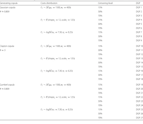
which may be tested on only one margin (to simplify the text). The censoring followed an exponential distribution such thatλs=15 =0.041,λs=30 =0.090 andλs=70 =0.308 where s represents the censoring percentage simulated. For all data generating processes (DGP), the Kendall’s tau was identical and represented an intermediate level of dependence between marginal distributions to be fair with the reality:τK =0.60. Then, we computed the right cop-ula parameter, for each copcop-ula, based on this Kendall’s tau. We also used a relatively standard mean and variance in cost-effectiveness analysis, following parameters used by Thompson and Nixon [13], such thatμC = 1500,σC = 400; μTadj = 4,σTadj = 0.75, and we parametrized each marginal distribution to keep close to these values. For the choice of generating copulas, we selected the three most-known ones with the biggest difference: Gaussian, Clayton and Gumbel copulas. The DGPs schemes is shown on Table 1.
The simulation of linearly dependent and uncensored covariates for costs leads to a bias in our advantage for the computation of the mean and the variance, com-pared to the estimation performed according to a standard clinical scheme. We decided therefore to challenge our method using the Kaplan-Meier mean estimate of the sur-vival function and its associated variance (which is the appropriate approach in absence of covariates of interest) instead of the presented procedure based on the covari-ates. Then, we applied the following steps: selecting a parametric distribution for the margins, selecting a para-metric copula using the information criterion and finally, looking for the copula parameter. We replicated this pro-cedure 500 times forn=1000 data, then we collected the provided information on the frequency of successful pro-cedures for the inference on the margins, the estimated Kendall’s tau and the choice of copula, respectively.
Inference on Kendall’s tau
Table 1Scheme of the 27 data generated cases
Generating copula Costs distribution Censoring level DGP
Gaussian copula FC∼N(μC=1500,σC=400) 15% DGP 1
θ≈0.809 30% DGP 2
70% DGP 3
FC∼(shapeC=12,scaleC=125) 15% DGP 4
30% DGP 5
70% DGP 6
FC∼logN(νC=7.30,τC=0.25) 15% DGP 7
30% DGP 8
70% DGP 9
Clayton copula FC∼N(μC=1500,σC=400) 15% DGP 10
θ=3 30% DGP 11
70% DGP 12
FC∼(shapeC=12,scaleC=125) 15% DGP 13
30% DGP 14
70% DGP 15
FC∼logN(νC=7.30,τC=0.25) 15% DGP 16
30% DGP 17
70% DGP 18
Gumbel copula FC∼N(μC=1500,σC=400) 15% DGP 19
θ≈0.809 30% DGP 20
70% DGP 21
FC∼(shapeC=12,scaleC=125) 15% DGP 22
30% DGP 23
70% DGP 24
FC∼logN(νC=7.30,τC=0.25) 15% DGP 25
30% DGP 26
70% DGP 27
Table 2Information on the estimation of the Kendall’s tau for each censoring level
Censoring level Mean(τˆK) Var(τˆK) Min(τˆK) Max(τˆK) Censoring =0% 0.6002 0.00019 0.5488 0.6476 Censoring =15% 0.6011 0.00024 0.5416 0.6539 Censoring =30% 0.6030 0.00035 0.5319 0.6648 Censoring =70% 0.6089 0.00146 0.4624 0.7257
The outputs of the 9 simulations with a censoring of 0% are joint together in the information on the first line and the same for simulations censored at 15% on the second line, 30% at the third line and 70% at the last line
as is the dispersion onτˆK, sinceτKranges in [−1, 1] while, for example, for Clayton copula,θranges in [−1,∞)\ {0}.
Inference on the marginal distribution for the costs
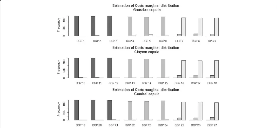
To select the right marginal distribution for costs on each of the 500 simulations and for each DGP, we used the proposed criteria based on the deviance. Thus, on Fig. 2, one can see the performance of this criterion. One may remark that, even with a 70% rate of censoring, the chosen parametric distribution is almost always correctly estimated.
Inference on the copula models
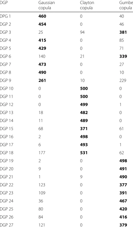
There exists a bunch of parametric copula families, but for the purpose of these simulations, we limited our selection to the most well-known ones: Gaussian, Stu-dent, Clayton, Gumbel, Frank and Joe copulas. However, with a real dataset, the reader may test any consistent
parametric copula using the proposed way. During sim-ulations, for each iteration, we collected the information about the selected family using the information criterion. At Tables 3 and 4, one can see these results for each DGP. We indicated, in bold, the copula that was selected the most in the 500 iterations and claimed that it was the copula to be retained for the mentioned DGP. When the selection of the copula was only in-between those used to simulate the data (as on Table 3), it was obvious that the chosen copula family is the one used for the generation process. Otherwise, when intermediate copulas (for which dependence adequation is close to the one provoked by the generating copula) are introduced in the selection pro-cess, the results may differ as shown on Table 4. For the DGPs where the costs were simulated following a normal distribution (1,2,3,10,11,12,19,20 and 21), the choice of the copula was influenced by the dependence caused by the type of copula retained to generate the data. In facts, when the costs margin followsN(μC = 1500,σC = 400)and the QALY margin follows N(μTadj = 4,σTadj = 0.75), usingτK =0.60, if the dependency distribution is mostly normal (i.e. comes from a Gaussian or a Gumbel copula), there will be a moderate tail on both tails of the distri-bution with an uniform cloud along the correlation path. For these reasons which are attributes of the Frank cop-ula, it was the chosen copula for DGPs 1,2,3,19,20 and 21. However, when, from the generating Clayton copula, a strict dependence was imposed to the left-tail while a mostly total independence was imposed to the right-tail, only a Clayton copula appeared appropriate to modeling
Fig. 2Frequency of selection of parametric marginal distributions for costs from the deviance criteria for each data generating process (DGP). The
black barrepresents the selection of the Normal distribution, thedark-gray barrepresents the selection of the Gamma distribution and thelight-gray
Table 3Frequency of choice of a copula for each DGP given 500 iterations for the three main copulas
DGP Gaussian Clayton Gumbel
copula copula copula
DPG 1 460 0 40
DGP 2 454 0 46
DGP 3 25 94 381
DGP 4 415 0 85
DGP 5 429 0 71
DGP 6 140 21 339
DGP 7 473 0 27
DGP 8 490 0 10
DGP 9 261 10 229
DGP 10 0 500 0
DGP 11 0 500 0
DGP 12 0 499 1
DGP 13 18 482 0
DGP 14 11 489 0
DGP 15 68 371 61
DGP 16 2 498 0
DGP 17 6 493 1
DGP 18 177 531 62
DGP 19 2 0 498
DGP 20 9 0 491
DGP 21 1 9 490
DGP 22 123 0 377
DGP 23 109 0 391
DGP 24 36 0 467
DGP 25 80 0 420
DGP 26 84 0 416
DGP 27 121 0 379
The chosen copula is in bold font
these data. That’s the reason why it was the chosen copula for DGPs 10,11 and 12. In the situation where QALY fol-lowsN(μE = 4,σE = 0.75)while costs follows a skewed marginal distribution (gamma or lognormal), in any case, there was not a right-tailed distribution, but mostly a left-oriented data cloud with a fat left-tail. That is the reason why, even when the data were generated from a Clayton copula, the Student (t) copula was the chosen one. There-fore, the simulations showed that the Bayesian criterion of selection of the copula was in accordance with the theoretical properties of the parametric copulas.
According to the structure of the marginal distributions, the choice of the copula could only be done in a limited spectrum of families. Therefore, when one seeks to find the best structural copula family, it appears essential to include the most known copula families covering as many
Table 4Frequency of choice of copula for each DGP on 500 iterations beyond the three main copulas and intermediate copulas
DGP Gaussian Student Clayton Gumbel Frank Joe copula copula copula copula copula copula
DPG 1 7 45 6 25 415 2
DGP 2 2 44 4 25 425 1
DGP 3 4 54 4 17 421 0
DGP 4 32 297 0 56 112 3
DGP 5 26 291 0 59 120 4
DGP 6 23 284 0 79 113 1
DGP 7 47 343 1 45 38 26
DGP 8 55 344 0 43 33 25
DGP 9 55 328 0 56 37 24
DGP 10 0 12 364 0 124 0
DGP 11 0 17 372 0 111 0
DGP 12 0 5 385 0 110 0
DGP 13 0 427 56 0 17 0
DGP 14 2 433 55 0 10 0
DGP 15 1 431 58 0 10 0
DGP 16 1 477 19 2 1 0
DGP 17 2 476 18 0 4 0
DGP 18 4 472 19 0 4 1
DGP 19 0 18 0 110 196 176
DGP 20 0 20 0 107 214 159
DGP 21 0 17 0 109 202 172
DGP 22 13 236 0 153 67 31
DGP 23 19 231 0 157 58 35
DGP 24 23 161 0 204 75 37
DGP 25 32 198 0 177 13 80
DGP 26 39 213 0 148 13 87
DGP 27 37 210 0 167 17 69
The chosen copula is in bold font
dependence states as possible. Thus, in harmony with Table 4, a selected copula which is not the generating one is only performing a better adequacy to the dependence between margins structures than the original one.
One remarks that an high censoring level does not really impact the issue of the copula estimation. Indeed, for all DGPs with 70% censoring level, there is only one case where the result changes: DGP 24. In fact, the Gumbel copula is left-skewed, as Student copula may be; which can explains the wrong estimation of the copula in this case.
Example: acupuncture for chronic headache in primary care data
Table 5Information gained in the analysis process for costs and QALY in both arms
Modelisation process Control arm Acupuncture arm
Kendall’s tau(τˆK) −0.1065 −0.1232
QALY distribution Tadj∼N(μˆTadj=0.7083,σˆTadj=0.1118) Tadj∼N(μˆTadj=0.7268,σˆTadj=0.1190)
Costs statistics μˆC=217.20 μˆC=403.40
ˆ
σC=486.00 σˆC=356.59
Costs distribution C∼logN(νˆC=4.4844,τˆC=1.3390) C∼logN(νˆC=5.7111,τˆC=0.7600)
Selected copula family Gaussian Student (t)
Copula parameter(θ)ˆ −0.1664 −0.1923
migraine and chronic tension headache of 401 patients aged 18 to 65 years old who reported an average of at least two headaches per month. Subjects were recruited in the general practice context in England and Wales and they were allocated to receive until 12 acupunc-ture treatments for a period of three months. For the sake of the study, acupuncture intervention was provided in the community by the United Kingdom National Health Service (NHS). The study starts in 2002 with a time horizon of 12 months and was registered ISRCTN96537534.
The data collection focuses on the measure of effective-ness in terms of QALY gained and the cumulative cost associated in UK pounds (£). Patients themselves reported unit costs associated with non-prescription drugs and pri-vate healthcare visits. The cost of the study intervention was estimated from the standard cost for a NHS profes-sional multiplied by the contact time with the patient. Thus, patients in the treated arm had a mean time of 4.2 hours with study acupuncturist. No imputation for missing data was done if the three questionnaires were not complete and consequently for which QALY cannot be measured. Therefore, in the acupuncture arm, there was 136 participants and in the control arm, 119. The modeling process of both joint distributions function for QALY and costs in the two clinical arms is presented on Table 5. We remark that in both cases, dependence is weak since that Kendall’s tau ranges between -0.10 and -0.15. Here, for the distribution of Tadj, we com-pared two possibles choices: a Gamma distribution and a gaussian one. The normal distribution has the small-est deviance. For the choice of distributions for costs, in the two arms, the lognormal distribution was con-sidered as the one with the smallest deviance. For the copula family selection using deviance information cri-teria, we compared, for each arm, Gaussian, Clayton, Student, Frank, Joe and Gumbel copulas. In the treated arm, Student copula was the considered one while in the control arm, it was the Gaussian copula. Therefore, the joint distribution function of the acupuncture arm was estimated by:
ˆ
F
Cj=1,Tadjj=1
=C(θˆStudent=− ) 0.1923
×FC∼logN
ˆ
νC=5.7111,τˆC=0.7600
,
FTadj∼N
ˆ
μTadj=0.7268,σˆTadj=0.1190
while, for the control arm, the estimation is:
ˆ
F
Cj=0,Tadjj=0
=Cθ(ˆGaussian=− ) 0.1664
×FC∼logN
ˆ
νC=4.4844,τˆC=1.3390
,
FTadj∼N
ˆ
μTadj=0.7083,σˆTadj=0.1118
.
Using the approach given from the copula densities, the ICER is estimated such thatICERˆ = 10082.68£/ unit of effectiveness, with a confidence interval which is:
ˆ
ICER ⎛ ⎜
⎝1+12.44z 2
1−α±z1−α/2
365336.81−9744.36×z2 1−α/2 1−z2
1−0.0266α/2
⎞ ⎟ ⎠
wherez1−αis the 100(1−α/2)percentile of the standard gaussian distribution. It means that it costs approximately 10082.68 per year to get an additional unit of effectiveness using acupuncture for headache.
The plot of the estimated INB with his 90 percent confidence limits versus lambda in presented on Fig. 3.
Table 6Information gained in the analysis process QALY in both arms, where an artificial censoring around 30 percents has been created
Modelisation process Control arm Acupuncture arm
Kendall’s tau(τˆK) −0.1388 −0.1011
QALY distribution Tadj∼N(μˆTadj=0.7133,σˆTadj=0.1026) Tadj∼N(μˆTadj=0.7304,σˆTadj=0.1005)
Selected copula family Gaussian Gaussian
Copula parameter(θ)ˆ −0.2163 −0.1582
The vertical intercept shows the negative value of the variability of costs and its confidence interval while the horizontal intercept shows the estimated ICER. Since the number of covariates was limited, it has not been pos-sible to determine the existence of subgroups. Whether available, the search for subgroups is possible using our approach.
Impact of an artificially created censoring on the acupuncture example
To challenge our methodology via a censored dataset, we decided to create an artificial censoring on QALY variable
(since that costs are assumed to always be observed). This censoring variable followed an exponential distribution where λ = 0.30. Hence, the QALY variable has been censored on approximately 30% of data. Using the same methodology than for the acupuncture original dataset, we obtained the information shown on Table 6. One notes that we did not report the costs information on this table since that it does not change from the information on Table 5 (costs is not a censored variable).Using these infor-mation, one obtains an estimated ICER such thatICERˆ =
10879.89£/ unit of effectiveness, with a confidence inter-val which is:
ˆ
ICER ⎛ ⎜
⎝1+11.33z 2
1−α±z1−α/2
360533.67−7443.98×z2 1−α/2 1−z2
1−0.0206α/2
⎞ ⎟ ⎠.
Hence, with a certain level of censoring, the estimation of ICER loses accuracy, and the confidence interval gets larger. However, the estimated ICER in case of censoring stay relatively close to the estimated ICER with original data, and stays in his confidence interval.
Synthesis on the acupuncture example
Firstly, let take a look at the conclusions of Wonderling et al. [36], who were the first to work on these original data. Without totally detailing their methodology, they used a linear regression adjusted on covariates of interest (age, sex, diagnosis, severity of headache at baseline, number of years of headache disorder, baseline SF-36 results and geographical site) to evaluate the mean difference for costs and effectiveness (in terms of QALY). Hence, from a lin-ear model, they have got an ICERˆ equals to 9180 £with a mean health gain for acupuncture treatment of 0.021 QALY.
Using the copula-based methodology presented in this paper, we get, with these original data, a mean health gain for acupuncture treatment of 0.026 QALY and when we apply an exponentially distributed censoring around 30% on QALY variable, we get a mean health gain for acupuncture treatment of 0.021 QALY. The major differ-ence between both approaches is on the estimated ICER value. However, we remark that the value of 9180 £keeps in the confidence interval of the copula-based ICER.
Conclusion
One motivation for this work was generated by the lim-itations of the at standard regression models applied to the cost-effectiveness analysis where the dependence structure between costs and utility along with time was not taken into account. We provided a simple step-by-step procedure to find INB and ICER and their confidence intervals, even in case of censoring.
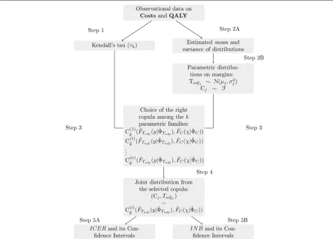
On Fig. 4, one sees the schematized method from the observational data produced by both clinical arms to the complete cost-effectiveness analysis. In a parallel way, one accomplishes steps 1 and 2 which are the measure of the dependence between QALY and cumulative costs in each arm via Kendall’s tau and the determination of the marginal distributions of both random variables. Then, at step 3, one generates copulas from information gained in steps 1 and 2 and, using the information criterion, one selects the closest copula to the right joint distribution function at step 4. Finally, at step 5, one determines the INB and the ICER using joint cdf. In case of subgroups cohorts analysis, one reiterate the procedure from step 1 to 5 to get two supplementary copulas and then, the joint
cdf of costs and QALY for the crossed-arms covariance terms.
The methodology presented here can easily be imple-mented on computational software. Indeed, on R, using the packagescopula[38] andCDVine[39], one can eas-ily apply the whole process to a dataset, either censored or not. OnSAS, the use of aPROC COPULAwill be enough to fit a certain copula on a whole dataset.
Appendix
Proposition 1The random variables Tadjji andηji are
dependent.
Proof To simplify the notation, let assume the
follow-ing befollow-ing for an individualion a therapeutic j. Also, let
Tadj(ω)=
T(ω)
0 Q(t)dt. Given the observed timesE(ω)= inf(η(ω),T(ω)). Ifη(ω)≤T(ω), one gets
Tadj(ω) =
η(ω)
0
Q(t)dt+
T(ω)
η(ω) Q(t)dt
= ηadj(ω)+ T(ω)
η(ω) Q(t)dt = ηadj(ω)+f(η(ω))
wheref is a function ofη(ω). Thus,Tadj(ω)is dependent ofη(ω).
Proposition 2The random variables Tadjjiandηadjjiare
independent.
Proof Let
Tadj(ω) =
T(ω)
0
Q(t)dt
= H[T(ω)]
and
ηadj(ω) = η(ω)
0
Q(t)dt
= H[η(ω)]
whereHis an invertible Borel function (hence monotone). Since thatT(ω)andη(ω)are independent, consequently
H[T(ω)] and H[η(ω)] are independent. Thus,Tadjji and ηadjjiare independent.
Proposition 3The random variables Cji and ηji are
dependent.
Proof To simplify the notation, let assume the following
be for an individualion a therapeutic armj. One has:
C(ω)=
T(ω)
0 Ck(t)dt ifT(ω)≤η(ω); η(ω)
Then, withE(ω)=inf(η(ω),T(ω)),
Ck(E(ω))=1[T(ω)≤η(ω)]C(T(ω))+1[η(ω)≤T(ω)]C(η(ω)).
Thus, assuming thatT(ω) is independent fromη(ω), one sees thatη(ω)andC(ω)are dependent.
Abbreviations
CEA: Cost-effectiveness analysis; DGP: Data generating process; DIC: Deviance information criterion; ICER: Incremental cost-effectiveness ratio; INB: Incremental net benefit; IPCW: Inverse probability censoring weighted; QALY: Quality adjusted life years
Acknowledgments
The authors wish to thank the National Health Society (UK), through the courtesy of Andrew J. Vickers, for allowing us to use the data on acupuncture for chronic headache in primary care data in this paper.
Funding
This research received no specific grant from any funding agency in the public, commercial, or not-for-profit sectors.
Availability of data and materials
Since the acupuncture data are not the property of the authors, they are not available through this article. However, they are available via the supplemental material of Vickers [37] on the link: https://www.ncbi.nlm.nih.gov/pmc/ articles/PMC1489946/bin/1745-6215-7-15-S1.xls.
Authors’ contributions
CF performed all simulations, statistical analysis, interpretations and drafted the article. Both CF and JPD designed the new methodology presented and the theoretical extensions. PL critically revised the article. All authors have read and approved the final manuscript.
Competing interests
The authors declare that they have no competing interests.
Consent for publication
Not applicable.
Ethics approval and consent to participate
Data are de-identified and authors got the authorization from Pr. A.J. Vickers for a secondary analysis of the data.
Received: 20 June 2016 Accepted: 2 February 2017
References
1. Willan A, Lin D. Incremental net benefit in randomized clinical trial. Stat Med. 2001;20:1563–74.
2. Kaplan E, Meier P. Nonparametric estimation from incomplete observations. J Am Stat Assoc. 1958;53:457–81.
3. Zhao H, Bang H, Wang H, Pfeifer PE. On the equivalence of some medical cost estimators with censored data. Stat med. 2007;26(24):4520–30. 4. Weinstein MC, Stason WB. Foundations of cost-effectiveness analysis for
health and medical practices. New England J Med. 1977;296(13):716–21. 5. Willan A, Chen E, Cook R, Lin D. Incremental net benefit in clinical trials
with quality-adjusted survival. Stat Med. 2003;22:353–62.
6. Willan A, Lin D, Manca A. Regression methods for cost-effectiveness analysis with censored data. Stat Med. 2005;24:131–45.
7. Pullenayegum E, Willan A. Semi-parametric regression models for cost-effectiveness analysis: Improving the efficiency of estimation from censored data. Stat Med. 2007;26:3274–99.
8. Sklar M. Fonctions de répartition àndimensions et leurs marges. Publ Inst Statist Univ Paris. 1959;8:229–31.
9. Embrechts P, McNeil A, Straumann D. Correlation and dependence in risk management: properties and pitfalls. Risk management: value at risk and beyond. 2002;176–223.
10. Frees EW, Valdez EA. Understanding relationships using copulas. North Am Actuar J. 1998;2(1):1–25.
11. Hougaard P. Analysis of multivariate survival data: Springer Science & Business Media; 2012.
12. Nelsen RB. An introduction to copulas. Springer Series in Statistics. New York: Springer; 2006.
13. Thompson S, Nixon R. How sensitive are cost-effectiveness analyses to choice of parametric distributions? Med Decision Making. 2007;4:416–23. 14. Stamey J, Beavers D, Faries D, Price K, Seaman J. Bayesian modeling of
cost-effectiveness studies with unmeasured confounding: a simulation study. Pharm Stat. 2014;13:94–100.
15. Lin D. Linear regression analysis of censored medical costs. Biostatistics. 2000;1:35–47.
16. Buckley J, James I. Linear regression with censored data. Biometrika. 1979;66:429–36.
17. Miller R, Halpern J. Regression with censored data. Biometrika. 1982;69-3: 521–31.
18. Genest C, Rivest LP. Statistical inference procedures for bivariate archimedean copulas. J Am Stat Assoc. 1993;88:1034–43.
19. Genest C, Ghoudi K, Rivest LP. A semiparametric estimation procedure of dependence parameters in multivariate families of distributions. Biometrika. 1995;82:543–52.
20. Brahimi B, Necir A. A semiparametric estimation of copula models based on the method of moments. Stat Method. 2012;9(4):467–77.
21. Kendall M. A new measure of rank correlation. Biometrika. 1938;30:81–9. 22. Oakes D. A concordance test for independence in the presence of
censoring. Biometrics. 1982;38:451–5.
23. Oakes D. On consistency of kendall’s tau under censoring. Biometrika. 2008;95-4:997–1001.
24. Lakhal-Chaieb L. Copula inference under censoring. Biometrika. 2010;97-2:505–12.
25. Dos Santos Silva R, Freitas Lopes H. Copula, marginal distributions and model selection: a bayesian note. Stat Comput. 2008;18:313–20. 26. Genest C, Neslehova J, Ben Ghorbal N. Estimators based on kendall’s tau
in multivariate copula models. Aust NZ J Stat. 2011;53:157–77. 27. El Maache H, Lepage Y. Spearman’s rho and kendall’s tau for multivariate
data sets. Math Stat Appl, Lect Notes-Monograph Series. 2003;42:113–30. 28. Fieller EC. Some problems in interval estimation. J Stat Royal Soc Ser B.
1954;16:175–85.
29. Willan A, O’Brien B. Confidence intervals for cost-effectiveness ratios: an application of fieller’s theorem. Health Econ. 1996;5:297–305.
30. Chaudhary N, Stearns S. Confidence intervals for cost-effectiveness ratios: an example from randomized trial. Stat Med. 1996;15:1447–58. 31. Siani C, Moatti JP. Quelles méthodes de calcul des régions de confiance
du ratio coût-efficacité incrémental choisir?: Universites d’Aix-Marseille II et III; 2002.
32. Bang H, Zhao H. Median-based incremental cost-effectiveness ratio (icer). J Stat Theory Prac. 2012;6(3):428–42.
33. Nixon R, Thompson S. Methods for incorporating covariate adjustment, subgroup analysis and between-centre differences into
cost-effectiveness evaluations. Health Econ. 2005;14:1217–29.
34. Tsai K-T, Peace KE, et al. Analysis of subgroup data in clinical trials. Journal of Causal Inference. 2013;1(2):193–207. De Gruyter.
35. Vickers AJ, Rees RW, Zollman CE, McCarney R, Smith CM, Ellis N, et al. Acupuncture for chronic headache in primary care: large, pragmatic, randomised trial. Bmj. 2004;328(7442):744.
36. Wonderling D, Vickers A, Grieve R, McCarney R. Cost effectiveness analysis of a randomised trial of acupuncture for chronic headache in primary care. British Med J. 2004;328:747–9.
37. Vickers AJ. Whose data set is it anyway? sharing raw data from randomized trials. Trials. 2006;7(1):15.
38. Kojadinovic I, Yan J, et al. Modeling multivariate distributions with continuous margins using the copula r package. J Stat Softw. 2010;34(9): 1–20.