16
Copyright © 2018. IJEMR. All Rights Reserved.
Volume-8, Issue-4, August 2018
International Journal of Engineering and Management Research
Page Number: 16-33
Process Capability Analysis in Single and Multiple Batch Manufacturing
Systems
Prof. Viraj V Atre
Faculty, Operations @ iFEEL – Institute for Future Education, Entrepreneurship and Leadership, Karla Lonavala District, Pune, INDIA
Corresponding Author: [email protected]
ABSTRACT
Any process, manufacturing or service in operations is subject to constant variation. The underlying principle of variation is any process / rather all processes are subject to changes occurring due to the magical 5 M’s that make the basis of operations management namely: Man, Machines, Materials, Methods and Money.
This paper discusses about establishment of a capable process, by means of stabilizing the 5 M’s and studying the variations which occur by going deeply into the well known term used in operations: RCA : Root Cause Analysis.
Keywords-- Process, Variation, Capability, Stability, Control, Statistical Process Control, Six Sigma Quality Root cause Analysis
I.
INTROCUTION
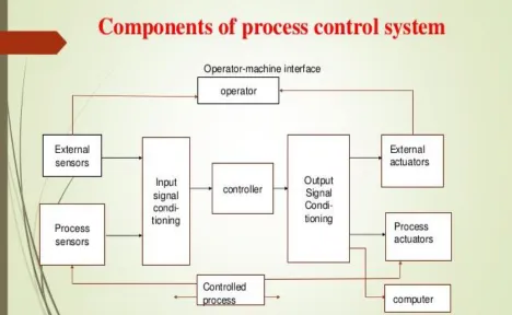
A. Process: A Process may be defined as an interconnected chain of various activities, which have to be done in chronological order. A Process may be a manufacturing process or a service process. Few examples like: airline and aeronautical operations, manufacturing an aircraft (it’s a big project) can be defined as a manufacturing process in sequential order. On the other hand, making pizza / burger with a sequential approach of ingredients, mixing, laying, marinating etc all the necessary activities as needed is a service process. Like manufacturing, food operations are also a service process. B. Variations: A process is subject to constant variations: let us consider a few examples of variations:
II.
MANUFACTURING & SERVICE
INDUSTRIES VARIATIONS
Manual variations: Operator skills, Operator Knowledge to operate a machine, Hand pressure on machine and machine tools, operating angle, tightening and loosing pressure on machine tools, holding procedures in jigs and fixtures, are all reasons behind end product variation caused. A simple Pressure on a drilling tool may make a hole or break the tool in the hands of the operator. A simple gas flame if not increased / decreased in the right manner may cause the taste of the food to change in the end. Lowering Down / increasing an Oxy-Acetylene Flame during gas Welding / gas cutting may have the impact on the welded joint / cut on the work in the long run. A simple way of applying an adhesive to two surfaces may create a strong bond or weak link on the materials joined, creating either a long term good effect or a leakage effect in the joint.
17
Copyright © 2018. IJEMR. All Rights Reserved.
need to identify the critical to quality parameters herewhich cause variation.
Machine variation: Machine variation is a common thing well accepted by the manufacturer as well as the buyer. No two machines manufactured from the same batch / assembly line will show the same results. The reasons are many, and are quite justified. Example; machine feed machine speed; rotational characteristics depend upon the input power supply. Variations in input power supply and frequency of the supply has a close impact on machine performance. Similarly, the operator handling the machine also has an impact on machine performance and variations. A simple example of driving a car at a constant speed without frequent change in gears, and applying frequent braking, may improve the mileage of the machine. That’s probably the only reason, why the same automobile will give different mileage to different drivers. It’s the same applicable in manufacturing / service industries, where different operators will get different results on the same machines they will operate. Numerous examples can be given on the combination of men, machines and materials in all the sectors of the industry.
Methodology / Technological variations: The method adopted by the man working on a certain machine, with a certain material is bound to some variation as different men will have different styles / methods of working. Speed, Accuracy, Precision, Linearity, Bias, Skills are the attributes which cause variations from men to men working on the same machines, same materials, same methodology. It is said that two men cannot work identically same, even if they fall in the super skilled category. However, by imparting proper training, and adopting a standard operating procedure (SOP) or Work instructional procedure (WI) these types of variations can be surely reduced.
Process Capability: A process has to go through three stages to make it a capable process in both the long and short run:
1. Process should be in Control 2. Process should be Stable
3. Process should be capable of producing the same results in short term and long term. 4. Process should be centered on the mean. Let us now understand Process Control, Process Stability, and Process capability through some diagrams
18
Copyright © 2018. IJEMR. All Rights Reserved.
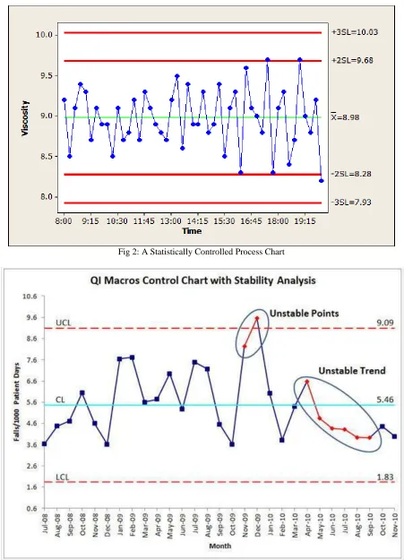
Fig 2: A Statistically Controlled Process Chart19
Copyright © 2018. IJEMR. All Rights Reserved.
Uncontrolled Process: Fig 3 above shows an uncontrolledprocess. As it may be seen from the graph points which have caused the process become unstable are showing an upward trend or a downward trend.
We usually plot time / quantity on the X axis (Horizontal scale) and measurements of the process on the Y axis (Vertical Scale).
Fig 2 above shows a controlled process statistically.
As it can be seen all the points measured lie within 3 sigma limits and no point has gone beyond UCL (upper control limit) or LCL (Lower control limit)
Stable and Controlled Process: Any Process is known to be in Control and Stable only if all the measurements points of the process are within Upper and Lower Control limits decided by the process controller. The Process is in control or not is measured by the formulae:
Capable Process: Any process is known to be Capable only if all the measured points in the process lie with USL (Upper Specification limits) and LSL (Lower Specification
20
Copyright © 2018. IJEMR. All Rights Reserved.
Process Capability Formulae21
Copyright © 2018. IJEMR. All Rights Reserved.
A Process Capability Analysis in MS-Excel22
Copyright © 2018. IJEMR. All Rights Reserved.
The recommended minimum or acceptable valueof Cp is 1.33. In terms of Six Sigma, this process capability is equivalent to a sigma level of 4 and long-term defect rate of 6,210 PPM. Process capability for a Six Sigma process is 2
Illustrative Example on Process Capability – 1 batch of 10 samples
A manufacturing process produced the following results of shafts manufactured of standard length of 125mm. the specification limits given by the customer are +/- 0.5 mm on either side
The Process is set at 3 sigma levels. We will now find the process capability of the existing process and also improve it by finding various measures of variation.
1
All 10 samples are taken so 100% inspection is done.
Let’s find process capability and control limits as follows:
Sr. No. Shaft Size (in mm)
1 124.86
2 124.94
3 124.95
4 124.89
5 125.02
6 125.01
7 125.03
8 124.88
9 125.05
10 124.69
Mean 124.932
Std.Dev. 0.108505
UCL 125.2575 USL Specified by Customer = 125.5
LCL 124.6065 LSL Specified by Customer = 124.5
Process Capability Cp = 1.536027636
Cpk upper Process Capability Ratio Cpk = 1.744927394
Cpk lower Process Capability Ratio Cpk = 1.327127877
23
Copyright © 2018. IJEMR. All Rights Reserved.
As we can see from the solved example above, astandard deviation of 0.10 has been achieved by reducing the variation by keeping specification limits of +/- of only 0.5mm on either side.
Further improvement can be achieved by reducing deviation limits to 0.25 mm on either side as well.
This clearly indicates, a small change in specification limits (reduction in variation) on either side
can improve process capability and subsequently sigma levels improvement.
Readers are requested to do the same calculations given above with specification limits (USL & LSL) of +/- 0.25 mm on either sides of the mean (125mm)
24
Copyright © 2018. IJEMR. All Rights Reserved.
Process Capability Report: Shaft Size (in mm)Count 10
Mean 124.93
StDev (Overall, Long Term) 0.108505
StDev (Within, Short Term) 0.097518
USL 125.5
Target
LSL
Capability Indices using Overall StDev
Pp
Ppu 1.74
Ppl
Ppk 1.74
Cpm
Potential Capability Indices using Within StDev
Cp
Cpu 1.94
Cpl
Cpk 1.94
Expected Overall Performance
ppm > USL 0.1
ppm < LSL
ppm Total 0.08259
% > USL 0.00%
% < LSL
% Total 0.00%
Actual (Empirical) Performance
% > USL
% < LSL
% Total 0.00%
Anderson-Darling Normality Test
A-Squared 0.417079
25
Copyright © 2018. IJEMR. All Rights Reserved.
Illustrative Example on Process Capability – 5 batches of 10 samplesA manufacturing process produced the following results of shafts manufactured of standard length of 125mm in 5 different batches produced. The specification limits given by the customer are 125mm +/- 0.5 mm on either side
The Process is set at 3 sigma levels. We will now find the process capability of the existing process of all the batches and do comparative analysis to improve it by finding various measures of variation.
Calculating Process Capability of Multiple Batches Samples for Six Sigma Analytics
Sample Batch 1 Batch 2 Batch 3 Batch 4 Batch 5
1 124.86 125.03 124.55 124.56 124.56
2 124.94 125.04 124.52 124.89 125.56
3 124.95 125.089 124.78 124.36 125.8
4 124.89 124.89 124.63 125.63 125.47
5 125.02 124.56 124.59 125.45 125.89
6 125.01 124.85 125.01 125.52 125.74
7 125.03 124.89 125.03 125.57 125.63
8 124.88 124.98 125.55 125.6 125.45
9 125.05 124.78 125.46 125.54 124.89
26
Copyright © 2018. IJEMR. All Rights Reserved.
Batch 1Count = 10 Mean = 124.93
StDev (Overall) = 0.108505 USL = 125.50
Target = LSL =
Capability Indices using Overall Standard Deviation Pp =
Ppu = 1.74 Ppl = Ppk = 1.74 Cpm =
Expected Overall Performance ppm > USL = 0.1
ppm < LSL = ppm Total = 0.1 % > USL = 0.00% % < LSL = % Total = 0.00%
Actual (Empirical) Performance % > USL = 0.00%
27
Copyright © 2018. IJEMR. All Rights Reserved.
Batch 2Count = 10 Mean = 124.87
StDev (Overall) = 0.175565 USL = 125.50
Target = LSL =
Capability Indices using Overall Standard Deviation Pp =
Ppu = 1.19 Ppl = Ppk = 1.19 Cpm =
Expected Overall Performance ppm > USL = 181.1
ppm < LSL = ppm Total = 181.1 % > USL = 0.02% % < LSL = % Total = 0.02%
Actual (Empirical) Performance % > USL = 0.00%
% < LSL = % Total = 0.00% USL = 125.5
0 2 4 6 8 10 12 4.36 12 4.62 12 4.87 12 5.13 12 5.38 12 5.64 12 5.89 Batch 1
28
Copyright © 2018. IJEMR. All Rights Reserved.
Batch 3Count = 10 Mean = 124.90
StDev (Overall) = 0.367848 USL = 125.50
Target = LSL =
Capability Indices using Overall Standard Deviation Pp =
Ppu = 0.55 Ppl = Ppk = 0.55 Cpm =
Expected Overall Performance ppm > USL = 50579.2
ppm < LSL = ppm Total = 50579.2 % > USL = 5.06% % < LSL = % Total = 5.06%
Actual (Empirical) Performance % > USL = 10.00%
29
Copyright © 2018. IJEMR. All Rights Reserved.
Batch 4Count = 10 Mean = 125.27
StDev (Overall) = 0.482498 USL = 125.50
Target = LSL =
Capability Indices using Overall Standard Deviation Pp =
Ppu = 0.16 Ppl = Ppk = 0.16 Cpm =
Expected Overall Performance ppm > USL = 319750.9
ppm < LSL = ppm Total = 319750.9 % > USL = 31.98% % < LSL = % Total = 31.98%
Actual (Empirical) Performance % > USL = 60.00%
30
Copyright © 2018. IJEMR. All Rights Reserved.
Batch 5Count = 10 Mean = 125.40
StDev (Overall) = 0.440153 USL = 125.50
Target = LSL =
Capability Indices using Overall Standard Deviation Pp =
Ppu = 0.08 Ppl = Ppk = 0.08 Cpm =
Expected Overall Performance ppm > USL = 407488.7
ppm < LSL = ppm Total = 407488.7 % > USL = 40.75% % < LSL = % Total = 40.75%
Actual (Empirical) Performance % > USL = 50.00%
31
Copyright © 2018. IJEMR. All Rights Reserved.
Process Capability Report: X-Bar: Batch 1 - Batch 5Count 50
Mean 125.07
StDev (Overall, Long Term) 0.398943
StDev (Within, Short Term) 0.403697
USL 125.50
Target
LSL
Capability Indices using Overall StDev
Pp
Ppu 0.36
Ppl
Ppk 0.36
32
Copyright © 2018. IJEMR. All Rights Reserved.
Potential Capability Indices using Within StDevCp
Cpu 0.35
Cpl
Cpk 0.35
Expected Overall Performance
ppm > USL 143242
ppm < LSL
ppm Total 143242.0
% > USL 14.32%
% < LSL
% Total 14.32%
Actual (Empirical) Performance
% > USL 24.00%
% < LSL
% Total 24.00%
33
Copyright © 2018. IJEMR. All Rights Reserved.
III.
CONCLUSION
This paper has been intended for understanding process capability analysis and calculations of how to establish a stable, controlled and capable process. By reducing process variations, a process can be controlled, stabilized and made capable in the long as well as short run. For a six sigma process, the capability metric Cp has to be 2 in the long run.
A simple formula used to compute sigma level from Cp or Cpk is as follows: Sigma level of a process = 3 * Cpk.
A usual practice is the Cpk should be 1 minimum so as to make a process at least 3 sigma level giving a 99.73% accuracy.
For a process to be 6sigma compliant the Cpk (Process capability ratio) must be 2
In this case paper the Process Capability achieved was 1.74 and has been further improved to 1.94 resulting in sigma level improvements from 5.22 to 5.82.
REFERENCES
[1] Bitran, G. R. & D. Tirupati. (1998). Planning and scheduling for epitaxial wafer production facilities. Operations Research, 36(1). 34-49.
[2] Bitran, G.R., E.A Haas, & A.C. Hax. (1981). Hierarchical production planning: A single stage system. Operations Research, 29, 717-743.