A General Solution to Einstein

(1)

International Journal of Sciences

Research Article

(ISSN 2305-3925)

Volume 2, Issue Apr 2013

http://www.ijSciences.com



Leandro Meléndez (Correspondence)



[email protected]

A General Solution to Einstein's

Equations in the Mixmaster Universe

Model

Leandro Meléndez

1 

, Pablo Chauvet

2 , Jaime Klapp

1

Instituto Nacional de Investigaciones Nucleares

2_{Universidad Autónoma Metropolitana - Iztapalapa}

Abstract:

Several papers have reported approximate solutions to Einstein's equations in the Mixmaster universe model. Through a specific scheme, a general solution is obtained here. A particular instance of this solution is also studied which proves to be equivalent to proposing from the start a Wick rotation intended to recreate the evolution of the Mixmaster cosmology in the Hartle-Hawking time.

Keywords

:

Einstein's equations, Cosmology, General Relativity

1. Introduction

The Bianchi IX anisotropic homogeneous models have played a key role in the theoretical cosmology of recent years [1]-[4]. These models were first studied and investigated in detail by Belinskii, Khalatnikov and Liftshitz (BKL) with an aim of exhibiting the generic form of the cosmological singularity in a spatially homogeneous anisotropic environment, as has been implied since General Relativity itself was introduced [5]-[10]. BKL find an approximate solution by introducing a simplification to Einstein's equations leading to a Bianchi IX abbreviated system [8]. Such an approximation describes the behaviour of a particle like universe in terms of collisions and other sudden changes of trajectory which entail a form of evolutive segregation of the universe scale factors [8],[9]. Simultaneously, and in a similar way, Misner studied the Bianchi IX model, introducing the term "Mixmaster cosmology" in order to describe his particular approach to the initial singularity suggesting an infinitely oscillating image in a supposedly chaotic form [11]-[13]. In fact, this model has been used in its classical form as an important example of the so-called "chaos in General Relativity" [14]-[18]. Misner includes a simplification to the model in the curvature anisotropy potential [11]. In contrast to BKL,

Misner resorts to the ADM (Arnowitt, Deser, Misner) technique to find that the model, in its presumed quantum-like form close to the singularity, and reproduces to a great extent the BKL results, namely, those of a particle colliding with a wall potential with intermediate stages identified as "Kasner" or "free particle" epochs [8],[11],[12]. Also in quantum terms, this universe model has been useful in exhibiting several propositions and consequences of the Hartle Hawking interpretation of the boundary conditions for physically acceptable solutions to the Wheeler-DeWitt equation [19],[20].

A substantial part of later studies, both theoretical and numerical [21]-[28], reproduce, to some extent, the concept of a universal particle colliding against a wall potential between free particle stages or "Kasner epochs" [8],[12].

More recently, an exact particular solution to the Mixmaster universe model within the complex General Relativity has been reported [29]. However, this solution restricts a particular value of one of the integral constants so as to simplify the process of finding a solution to the Einstein equations. This result is meant to resolve the long discussed integrability of the Bianchi IX model [30].

(2)

http://www.ijSciences.com Volume 2, Issue Apr 2013

55

Mixmaster Universe Model within complex

General Relativity, and the method to accomplish this solution. An interesting instance of this solution has also been included.

2. The Mixmaster Universe Model; First Derivatives

The scale factor evolution in the vacuum diagonal Bianchi IX (Mixmaster) cosmological model is governed by Einstein's field equations and a constraint, which are usually written as [5],[8],[9]:

 









0

2

1

1 ₄ ₂ ₂ 2





















a

c

b

abc

c

dt

db

a

dt

d

 









0

2

1

1 ₄



₂



₂ 2



















c

b

a

abc

bc

dt

da

dt

d

(1)

 









0

2

1

1 ₄



₂



₂ 2



















b

a

c

abc

dt

dc

ab

dt

d

0

2 2 1 2 2 1 2 2

1













c

dt

d

c

b

dt

d

b

a

dt

d

a

(2)

Then, with an aim of rewriting Einstein's field equations in a more compact manner in order to apply our above-mentioned method, we define the transformation:

 

2 

,

exp

 

2 

,

exp

 

2 

exp

2 2

2



c

b

a

(3)

j

₁



exp

 

2 



exp

 

2 



exp

 

2 

 

2 

exp

 

2 

exp

 

2 

exp

2





j

(4)

 

2 

exp

 

2 

exp

 

2 

exp

3









j

and



d

V

dt



(5) where

abc

V



(6)

by substituting this transformation in equations (1), one obtains that

3 1 2

2

2 j

j

d

_

_



2 1 2

2

2 j

j

d

_

_



(7)

3 2 2

2

2 j

j

d

_

_

_



A first integral of this system is equation (2), which can be written as [8]



2 3



1 3 2

2

2 j

j

d



















_



























_



















(8)

This equation is, in fact, a constraint on any solution to the second derivatives equation system. In the present case, despite having achieved a first integral, a solution to the second integral is still far from immediate, given the

scrambled first derivatives.

(3)

56 

dh

d





h



dh

d





h

i j

/

i k

/









,

where

h

_i,

h

_j and

h

_k can be any of

2 

,

2 

,



2

. Trivial solutions aside, one possible separation of the first derivatives seems to be

2

2 i

j

d

_

_



3

2 i

j

d

_

_



(9)

1

2 i

j

d

_

_

_



where

i





1

.

In order to show that this separate expression of the first derivatives satisfies Einstein's dynamical equations, let us consider, for instance, the derivative of the second equation of system (9) given by

 















































































d

i

d

2

2 exp

2

2 exp

2

2 exp

2

₂ 2 (10)

By substituting definitions (4) and the first derivatives apparent in (9), equation (10) can be written as:

2 1 2

2

2 j

j

d

_

_



It is clear now that equations (9) satisfy the second equation (7). Likewise, the other two equations (9) can be derived to verify that they satisfy the remaining equations (7). Hence, this fruitful analysis has led to a first integral of Einstein's Mixmaster universe model, now with separate expressions of the first derivatives.

3. A General Solution to the Mixmaster Universe

Obtaining a general solution to Einstein's equations for the Mixmaster cosmology takes us

to the

j

function space defined in the equation system (4), which turn out to be the Jacobi functions. To this purpose, equations (9) are substituted in (7), resulting in a new system in terms of the functions

j

₁,

j

₂ and

j

₃ instead of



,



and



, namely,

3 2 1

i

j

d

_

_



3 1 2

i

j

d

_

_



(11)

2 1 3

i

j

d







This equation system is strictly different to that reported by Belinskii et al. (BGPP) [6]. By multiplying each equation (11) by an adequate factor, one finds that

3 3 2 2 1 1

j

d

j

d

j

d

j





(12)

In other words, the squared functions

j

only differ from one another by an additive constant, so that

2 2 2 3 2 1 2 1 2 2 2 1

q

j

q

j









(13)

(4)

57

say





2



2 2 1 2 1 2 1

1

i

j

q

j

q

j

d















(14)

By integrating (14), one obtains





_

















2 2 2 1 0 2 1 1

,

q

iq

JacobiSN

q

j



(15)

where



₀,

q

₁ and

q

₂ are integration constants. Then, placing equation (15) in system (13), two expressions for

j

₂ and

j

₃ are arrived at which, along with

j

₁ from (15), satisfy equation system (11). Given the definitions of these functions along with expressions (4) and (3)

 

2 



/

2 exp

1 3

2

j

a









 

2 



/

2 exp

1 2

2

j

b









(16)

 

2 



/

2 exp

2 3

2

j

c











In this way, a general solution to Einstein's equations for the Mixmaster universe model has been obtained without any approximation. As we have seen, the

j

functions are complex and dependent on a complex variable. When analyzing them, it seems improbable that real or complex



or

q

₁,

q

₂ values exist that produce real scale factors and cosmological time.

In any case, assuming randomness, it is most probable that the variables and parameters involved take complex values. Thus, the need for conditions of reality is clear, which will be discussed in the next section. Meanwhile, the traditional real four-dimensional space-time appears to be different, namely, its entities involved now exhibit a complex nature, each one

of them possesses two degrees of freedom, both in space and in time. The

traditional classical four-dimensional scenery now encompasses eight dimensions.

4. Reality Conditions

Imposing some reality conditions on complex General Relativity is a rarely studied topic. However, logarithmic time values



and parametric values

q

₁,

q

₂ ensuring real cosmological time and scale factors, lead to find, at least, one conditions for a real cosmological time.

To this purpose, given the complexity of the mentioned values, it should be specified that

2 1







i

(17) In this new environment, with the squared scale factors in equations (16), equation (6) now looks like



1 2



2



1 2



1 2 2 2

,



iv

v

c

b

a

V









(18) and equation (5) becomes











v



iv





d



t

C







1 1

,

2 2 1

,

2 (19)

In this manner, equation (18) is integrated along a contour

C

on the plane



₂vs



₁. A reality condition for the cosmological time in equation (19) is, then,



1

,

2



1 2



1

,

2



2

0

1









C C

d

v

d

v



(20)

Notice that both the scale factors and expression (6) are complex functions of complex variables. The previous reality condition applies to the cosmological time alone. In the next section, an alternative imaginary cosmological time scenario is proposed.

5. The Imaginary Time

(5)

58

parameters

q

₁,

q

₂ to be purely imaginary, i.e.,

iT





1 1

ip

q



(21)

2 2

ip

q



and, where it is convenient, proposing that the real numbers

p

₁ and

p

₂ are related in such a way that 2

2 2 1

p



. Further simplifications are possible if also



₀



0

. Then, with expressions (21) substituted in equation (15) one finds

]

/

,

[

₂ ₁2 ₂2

1

i

p

JacobiSN

i

p

T

p

j



(22) Within this framework, it is possible to see that

j

₁ is a real function of real variables. Moreover, given expression (22) and equations (16), the squared scale factors can be put in the form:



22



/

2

2 1 1 2

p

j

a







12



/

2

2 1 1 2

p

j

b





(23)



22



/

2

2 1 2

1 2 1 2

p

j

p

j

c





These expressions turn out to be positive real functions under the conditions imposed on



,

q

₁, and

q

₂. Thus,

V



abc

is also a real function. Consequently, once such real functions are substituted in (5), the cosmological time becomes imaginary.

(6)

59

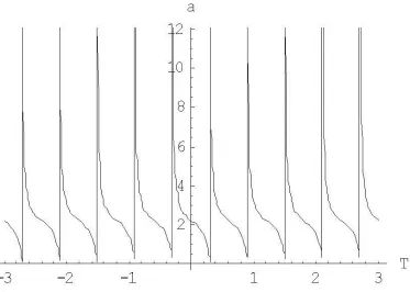
Figure 1. The time evolution of scale factor

a

for the Mixmaster universe general solution, when the

(7)

60

Figure 2. The scale factor

b

time evolution, for the Mixmaster universe general solution, when the

(8)

61

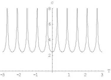
Figure 3. The scale factor

c

time evolution, for the Mixmaster universe general solution, when the

logarithmic time



and the parameters

q

1_and

q

2_{are purely imaginary. The curve shown in} this graphic is determined by

p

1



2

_and

p

2



10

It can be easily shown that solving the particular case determined by when the scale factors and equation (6) are real functions of pure imaginary variables can be alternatively achieved from applying a Wick



t



it



rotation from the beginning, leading to the evolution of the Mixmaster cosmology in the imaginary Hawking time.

6. Comments and Conclusions

Following a strategy applied to handling the expressions compacted in section 2, Einstein's equations for the Mixmaster universe model have been integrated, and an exact general solution has been found. Furthermore, this strategy enables one to translate the problem to the Jacobi function space, reducing the original formulation based upon three non-trivial Einstein's field equations and one constraint down to a single equation (14). To cap it all, the found solution is still more

general than the ones previously reported [5]-[10],[11],[29].

(9)

62

Finally, and coming back to the found general

solution, it is clear that its description of the universe evolution in the Mixmaster model is far more complicated than the conventional descriptions. This is mainly due to a change in the location of events from four to eight dimensions while the scale factors and the time exhibit two degrees of freedom each, bringing about a more sophisticated cosmology.

References

[1] J D Barrow, Nucl. Phys. B 296 697 (1988).

[2] M Carmeli and R Manor, Int. Jour. Theor. Phys. B

29[5] 521 (1990).

[3] W A Wright and I G Moss, Phys. Lett. B 154[2,3] 115 (1985).

[4] P S Apostolopoulos and M Tsamparlis, Gen. Rel. Grav.35[11] 2007 (2003).

[5] V A Belinskii and I M Khalatnikov, Sov. Phys.

J.E.T.P. 30[6] 1174 (1970).

[6] V A Belinskii, G W Gibbons, D N Page and C N Pope, Phys. Lett. B 76[4] 433 (1978).

[7] V A Belinskii, I M Khalatnikov and E M Lifshitz,

Phys. Lett.77A[4] 214 (1980).

[8] V A Belinskii, I M Khalatnikov and E M Lifshitz,

Adv. Phys.19 525 (1970).

J.E.T.P. 29[5] 911 (1969).

J.E.T.P. 32[1] 169 (1969).

[11] Ch W Misner, Phys. Rev. Lett.22A[20] 1071 (1969). [12] Ch W Misner, Phys. Rev..186[5] 1319 (1969). [13] A G Doroshkevich, V N Lukash and I D Novikov, ,

Sov. Phys. J.E.T.P. 33[4] 649 (1971).

[14] A Latifi, M Musette, R Conte, Phys. Lett. A 194 83 (1994).

[15] J D Barrow, Phys. Rev. Lett.46[15] 963 (1981). [16] J D Barrow, Phys. Reports (Rev. Sect. Of Phys. Lett.)

85[1] 1 (1982).

[17] D F Chernoff and J D Barrow, Phys. Rev. Lett.50[2] 134 (1983).

[18] N J Cornish and J J Levin, Phys. Rev. Lett.78 998 (1997).

[19] J Hartle and S Hawking, Phys. Rev. D 28 2960 (1983).

[20] O Obregón, J Pullin and M P Ryan, Phys. Rev. D

48[12] 5642 (1993).

[21] R A Matzner, L C Shepley and J B Warren, Ann. Phys.57 401 (1970).

[22] M P Ryan, Ann. Phys.65 506 (1971). [23] M P Ryan, Ann. Phys.68 541 (1971).

[24] R Moser, R A Matzner and M P Ryan, Ann. Phys. NY

79 558 (1973).

[25] K Ferraz and G Francisco, Phys. Rev. D 45[4] 1158 (1992).

[26] S E Rugh and B J T Jones, Phys. Lett. A 147 353 (1990).

[27] B K Berger, Gen. Rel. Grav.23 1385 (1991). [28] A Zardecki, Phys. Rev. D 28 1235 (1983).

[29] L Meléndez and P Chauvet, Gen. Rel. Grav.35[11] 2007 (2003).