A EFFICIENT COMPUTATIONAL METHOD FOR SOLVING
STOCHASTIC IT ˆO-VOLTERRA INTEGRAL EQUATIONS
FAKHRODIN MOHAMMADI1, §
Abstract. In this paper, a new stochastic operational matrix for the Legendre wavelets is presented and a general procedure for forming this matrix is given. A computational method based on this stochastic operational matrix is proposed for solving stochastic Itˆo-Voltera integral equations. Convergence and error analysis of the Legendre wavelets basis are investigated. To reveal the accuracy and efficiency of the proposed method some numerical examples are included.
Keywords: Legendre wavelets, Itˆo integral, Stochastic operational matrix, Stochastic Itˆo-Volterra integral equations
AMS Subject Classification: 65T60, 60H20
1. Introduction
Random or stochastic integrals are very important for modeling many phenomena in physics, mechanics, medical, finance, sociology, biology, etc. So many studies have been appeared in the recent literature which describe these stochastic mathematical models rather than deterministic ones. In many cases such phenomena dependent on a Gaussian white noise that mathematically are modeled as stochastic differential equations, stochastic integral equations or stochastic integro-differential equations of the Itˆo type [1–7].
Similar to the deterministic case, most stochastic differential and integral equation cannot be solved analytically and therefore numerical solution becomes a practical way to face this difficulty. Recently, there has been a growing interest in numerical solutions of stochastic differential and integral equations [1, 3–10].
Recently, different orthogonal basis functions, such as block pulse functions, Walsh func-tions, Fourier series, orthogonal polynomials and wavelets, were used to estimate solutions of functional equations. As a powerful tool, wavelets have been extensively used in sig-nal processing, numerical asig-nalysis, and many other areas. Wavelets permit the accurate representation of a variety of functions and operators [11, 12]. Legendre wavelets have been widely applied in system analysis, system identification, optimal control and numer-ical solution of integral and differential equations [13–16]. In this paper, an stochastic operational matrix for Legendre wavelets is derived. Then application of this stochas-tic operational matrix in solving stochasstochas-tic Itˆo-Voltera integral equation is investigated. Illustrative examples are included to demonstrate the validity and applicability of the technique.
1 Department of Mathematics, Hormozgan University, P. O. Box 3995, Bandarabbas, Iran. e-mail: [email protected];
§ Manuscript received: December 12, 2014.
TWMS Journal of Applied and Engineering Mathematics, Vol.5, No.2; cI¸sık University, Department of Mathematics, 2015; all rights reserved.
This paper is organized as follows: In section 2 some basic definition and preliminar-ies about stochastic process and Itˆo integral are presented. The Legendre wavelets and their properties are discussed in section 3. In section 4 stochastic operational matrix for Legendre wavelets and a general procedure for deriving this matrix are introduced. In sec-tion 5 applicasec-tion of this stochastic operasec-tional matrix in solving stochastic Itˆo-Volterra integral equations are described. Finally, a conclusion is given in section 7.
2. Preliminaries
In this section we review some basic definition of the stochastic calculus and the block pulse functions (BPFs).
2.1. Stochastic calculus.
Definition 2.1. (Brownian motion process) A real-valued stochastic process B(t), t ∈ [0, T] is called Brownian motion, if it satisfies the following properties
(i) The process has independent increments for0≤t0 ≤t1 ≤...≤tn≤T,
(ii) For all t≥0, B(t+h)−B(t) has Normal distribution with mean 0 and variance h, (iii) The function t→B(t) is continuous functions of t.
Definition 2.2. Let {Nt}t≥0 be an increasing family of σ-algebras of subsets of Ω. A process g(t, ω) : [0,∞) ×Ω → Rn is called Nt-adapted if for each t ≥ 0 the function
ω→g(t, ω) isNt-measurable.
Definition 2.3. Let V =V(S, T) be the class of functions f(t, ω) : [0,∞)×Ω→R such that
(i) The function(t, ω) →f(t, ω) is B × F-measurable, whereB denotes the Borel algebra on[0,∞) andF is theσ -algebra on Ω.
(ii) f is adapted to Ft, where Ft is the σ -algebra generated by the random variables
B(s), s≤t. (iii)E
RT
S f2(t, ω)dt
<∞.
Definition 2.4. (The Itˆo integral) Letf ∈ V(S, T), then the Itˆo integral of f is defined by
Z T
S
f(t, ω)dBt(ω) = lim n→∞
Z T
S
ϕn(t, ω)dBt(ω), (limin L2(P))
where, ϕn is a sequence of elementary functions such that
E
Z T
s
(f(t, ω)−ϕn(t, ω))2dt
→0, as n→ ∞.
For more details about stochastic calculus and integration please see [2].
2.2. Block pulse functions. BPFs have been studied by many authors and applied for solving different problems. In this section we recall definition and some properties of the block pulse functions [3, 17].
The m-set of BPFs are defined as
bi(t) =
1 (i−1)h ≤t < ih
0 otherwise (1)
in which t∈ [0, T), i= 1,2, ..., mand h = mT. The set of BPFs are disjointed with each other in the interval [0, T) and
where δij is the Kronecker delta. The set of BPFs defined in the interval [0, T) are
orthogonal with each other, that is
Z T
0
bi(t)bj(t)dt=hδij, i, j = 1,2, ..., m. (3)
Ifm → ∞the set of BPFs is a complete basis for L2[0, T), so an arbitrary real bounded function f(t), which is square integrable in the interval [0, T), can be expanded into a block pulse series as
f(t)'
m X
i=1
fibi(t), (4)
where
fi =
1 h
Z T
0
bi(t)f(t)dt, i= 1,2, ..., m. (5)
Rewritting Eq. (37) in the vector form we have
f(t)'
m X
i=1
fibi(t) =FTΦ(t) = ΦT(t)F, (6)
in which
Φ(t) = [b1(t), b2(t), ...., bm(t)]T, F = [f1, f2, ...., fm]T. (7)
Morever, any two dimensional functionk(s, t)∈L2([0, T1]×[0, T2]) can be expanded with respect to BPFs such as
k(s, t) = ΦT(t)KΦ(t), (8) where Φ(t) is the m-dimensional BPFs vectors respectively, and K is the m×m BPFs coefficient matrix with (i, j)-th element
kij =
1 h1h2
Z T1
0
Z T2
0
k(s, t)bi(t)bj(s)dtds, i, j= 1,2, ..., m, (9)
andh1= Tm1 and h2= Tm2. Let Φ(t) be the BPFs vector, then we have
ΦT(t)Φ(t) = 1, (10)
and
Φ(t)ΦT(t) =
b1(t) 0 . . . 0 0 b2(t) . .. ...
..
. . .. . .. 0 0 . . . 0 bm(t)
m×m
. (11)
For anm-vector F we have
Φ(t)ΦT(t)F = ˜FΦ(t), (12) where ˜F is anm×mmatrix, and ˜F =diag(F). Also, it is easy to show that for anm×m matrixA
3. Legendre wavelets
Wavelets constitute a family of functions constructed from dilation and translation of a single function ψ called the mother wavelet. When the dilation parameter a and the translation parameter b vary continuously, we have the following family of continuous wavelets
ψa,b(t) =a−
1 2ψ
t−a b
, a, b∈R, a6= 0. (14)
The Legendre wavelets are defined on the interval [0,1) as
ψmn(t) = ( q
m+122k+12 pm 2k+1t−(2n−1) n 2k ≤t <
n+1 2k
0 otherwise, (15)
wheren= 0,1, ...,2k−1 andm= 0,1,· · ·, M−1 is the degree of the Legendre polynomials for a fixed positive integer M. Here Pm(t) are the well-known Legendre polynomials of
degree m[13, 15].
Any square inegrable function f(x) defined over [0, 1) can be expanded in terms of the extended Legendre wavelets as
f(x)'
∞
X
n=0
∞
X
m=0
cnmψnm(x) =CTΨ(x), (16)
wherecmn= (f(t), ψmn(t)) and (., .) denotes the inner product onL2[0,1]. If the infinite
series in (16) is truncated, then it can be written as
f(x)' 2k−1
X
n=0
M−1
X
m=0
cmnψmn(x) =CTΨ(x), (17)
whereC and Ψ(x) are ˆm= 2kM column vectors given by
C=hc00, . . . , c0(M−1)|c10, . . . , c1(M−1)|, . . . ,|c(2k−1)0, . . . , c(2k−1)(M−1) iT
, (18)
Ψ(x) =hψ00(x), . . . , ψ0(M−1)(x)|ψ10(x), . . . , ψ1(M−1)(x)|, . . . ,|ψ(2k−1)0(x), . . . , ψ(2k−1)(M−1)(x) iT
.
By changing indices in the vectors Ψ(x) and C the series (17) can be rewritten as
f(x)' ˆ
m X
i=1
ciψi(x) =CTΨ(x), (19)
where
C= [c1, c2, ..., cmˆ], Ψ(x) = [ψ1(x), ψ2(x), ..., ψmˆ(x)], (20) and
ci =cnm, ψi(x) =ψnm(x), i= (n−1)M +m+ 1. (21)
Similarly, any two dimensional function k(s, t) ∈ L2([0,1]×[0,1]) can be expanded into Legendre wavelets basis as
k(s, t)≈ ˆ
m X
i=1 ˆ
m X
j=1
kijψi(s)ψj(t) = ΨT(s)KΨ(t), (22)
3.1. Relation between the BPFs and Legendre wavelets. In this section we will derive the relation between the Legendre wavelets and BPFs. It is worth mention that here we setT = 1 in definition of BPFs.
Theorem 3.1. Let Ψ(t) and Φ(t) be the m-dimensional Legendre wavelets and BPFsˆ vector respectively, the vector Ψ(t) can be expanded by BPFs vector Φ(t) as
Ψ(t)'QΦ(t), (23)
where Q is an mˆ ×mˆ block matrix and
Qij =ψi
2j−1 2 ˆm
, i, j= 1,2, ...,mˆ (24)
Proof. Letφi(t), i= 1,2, ...,mˆ be thei-th element of Legendre wavelets vector. Expanding
φi(t) into an ˆm-term vector of BPFs, we have
ψi(t)'
ˆ
m X
i=1
Qijbj(t) =QTiΦ(t), i= 1,2, ...,m,ˆ (25)
where Qi is the i-th row and Qij is the (i, j)-th element of matrix Q. By using the
orthogonality of BPFs we have
Qij =
1 h
Z 1
0
ψi(t)bj(t)dt=
1 h
Z j
ˆ m
j−1 ˆ m
ψi(t)dt= ˆm Z j
ˆ m
j−1 ˆ m
ψi(t)dt, (26)
by using mean value theorem for integrals in the last equation we can write
Qij = ˆm
j ˆ m−
j−1 ˆ m
ψi(ηi) =ψi(ηj), ηj ∈
j−1 ˆ m ,
j ˆ m
, (27)
now by choosingηj = 2j2 ˆ−m1 so we have
Qij =ψi
2j−1 2 ˆm
, i, j= 1,2, ...,m.ˆ (28)
and this prove the desired result.
The following Remark is the consequence of relations (12), (13) and Theorem 3.1.
Remark 3.1. For an m-vectorˆ F we have
Ψ(t)ΨT(t)F = ˜FΨ(t), (29)
in which F˜ is an mˆ ×mˆ matrix as ˜
F =QF Q¯ −1, (30) where F¯ =diag QTF
. Moreover, it can be easy to show that for anmˆ ×mˆ matrixA
ΨT(t)AΨ(t) = ˆATΨ(t), (31)
3.2. Convergence and error analysis. Here we investigate the convergence and error analysis of the Legendre wavelets basis.
Theorem 3.2. Let f(x) be a function defined on [0,1) with bounded second derivatives, say|f00(x)| ≤M, andP∞
n=0
P∞
m=0cmnψmn(x) be its infinite Legendre wavelets expansion, then
|cmn| ≤
√ 12M (2n)52(2m−3)2
, (32)
this means the Legendre wavelets series converges uniformly tof(x) and
f(x) =
∞ X n=1 ∞ X m=0
cnmψnm(x), (33)
Proof. See [18].
Theorem 3.3. Supposef(x)be a continuous function defined on[0,1), with second deriva-tives f00(x) bounded by M, then we have the following accuracy estimation
keM,k(t)k2 ≤ 3M 2 2 ∞ X n=0 ∞ X
m=M
1
n5(2m−3)4 + 3M2
2
∞
X
n=2k
M−1
X
m=0
1 n5(2m−3)4
!12
, (34)
where
keM,k(t)k2 =
Z 1
0
f(x)−
2k−1 X
n=0
M−1
X
m=0
cnmψnm(x) 2 dx 1 2 .
Proof. We have:
σM,k2 =
Z 1 0
f(x)−
2k−1
X
n=0
M−1
X
m=0
cnmψnm(x) 2 dx = Z 1 0 ∞ X n=0 ∞ X m=0
cnmψnm(x)−
2k−1 X
n=0
M−1
X
m=0
cnmψnm(x) 2 dx = ∞ X n=0 ∞ X
m=M
c2nm
Z 1
0
ψnm2 (x)dx+
∞
X
n=2k
M−1
X
m=0 c2nm
Z 1
0
ψnm2 (x)dx=
∞
X
n=0
∞
X
m=M
c2nm+
∞
X
n=2k
M−1
X
m=0 c2nm, now by considering Eq. (32), the desired result is achieved.
4. Stochastic operational matrix of Legendre wavelets
In this section we obtain the stochastic integration operational matrix for Legendre wavelets. For this purpose we first remind some useful results for BPFs [3, 4].
Lemma 4.1. [3] Let Φ(t) be them-dimensional BPFs vector defined in (7), then integra-ˆ tion of this vector can be derived as
Z t
0
where P is called the operational matrix of integration for BPFs and is given by
P = h 2
1 2 2 . . . 2 0 1 2 . . . 2 0 0 1 ... ...
..
. ... ... . .. 2 0 0 0 . . . 1
ˆ
m×mˆ
. (36)
Lemma 4.2. [3] LetΦ(t)be them-dimensional BPFs vector defined in (7), the Itˆˆ o integral of this vector can be derived as
Z t
0
Φ(s)dB(s)'PsΦ(t), (37)
where Ps is called the stochastic operational matrix of BPFs and is given by
Ps=
B h2 B(h) B(h) . . . B(h) 0 B 32h−B(h) B(2h)−B(h) . . . B(2h)−B(h)
0 0 B 52h
−B(2h) . . . B(3h)−B(2h) ..
. ... ... . .. ...
0 0 0 . . . B(2 ˆm2−1)h−B(( ˆm−1)h)
ˆ
m×mˆ .
Now we are ready to derive a new operational matrix of stochastic integration for the Legendre wavelets basis. For this end we use BPFs and the matrixQintroduced in (23).
Theorem 4.1. Suppose Ψ(t) be the m-dimensional Legendre wavelets vector defined inˆ (20), the integral of this vector can be derived as
Z t
0
Ψ(s)ds'QP Q−1Ψ(t) = ΛΨ(t), (38) where Q is introduced in (23) and P is the operational matrix of integration for BPFs derived in (36).
Proof. Let Ψ(t) be the Legendre wavelets vector, by using Theorem 3.1 and Lemma 4.1 we have
Z t
0
Ψ(s)ds'
Z t
0
QΦ(s)ds=Q
Z t
0
Φ(s)ds=QPΦ(t), (39)
now Theorem 3.1 give
Z t
0
Ψ(s)ds'QPΦ(t) =QP Q−1Ψ(t) = ΛΨ(t), (40)
and this complete the proof.
Theorem 4.2. Suppose Ψ(t) be the m-dimensional Legendre wavelets vector defined inˆ (20), the Itˆo integral of this vector can be derived as
Z t
0
Ψ(s)dB(s)'QPsQ−1Ψ(t) = ΛsΨ(t), (41)
where Λs is called stochastic operational matrix for Legendre wavelets, Q is introduced in
Proof. Let Ψ(t) be the Legendre wavelets vector, by using Theorem 3.1 and Lemma 4.2 we have
Z t
0
Ψ(s)dB(s)'
Z t
0
QΦ(s)dB(s) =Q
Z t
0
Φ(s)dB(s) =QPsΦ(t), (42)
now Theorem 3.1 result
Z t
0
Ψ(s)dB(s) =QPsΦ(t) =QPsQ−1Ψ(t) = ΛsΨ(t), (43)
and this complete the proof.
5. Application in solving stochastic integral equations
In this section, we solve stochastic Itˆo-Volterra integral equations by using the stochastic operational matrix of the Legendre wavelets. Consider the following stochastic Itˆo-Volterra integral equation as
X(t) =f(t) +
Z t
0
k1(s, t)X(s)ds+
Z t
0
k1(s, t)X(s)dB(s), t∈[0, T), (44)
whereX(t),f(t),k1(s, t) andk2(s, t), fors, t∈[0, T), are the stochastic processes defined on the same probability space (Ω, F, P), andX(t) is unknown. AlsoB(t) is a Brownian mo-tion process andR0tk1(s, t)X(s)dB(s) is the Itˆo integral. For solving this problem by using the stochastic operational matrix of Legendre wavelets, we approximateX(t), f(t), k1(s, t) andk2(s, t) in terms of ˆm-dimentional Legendre wavelets as follows
f(t) =FTΨ(t) = ΨT(t)F, (45)
X(t) =XTΨ(t) = ΨT(t)X, (46)
k1(s, t) = Ψ(s)TK1Ψ(t) = Ψ(t)TK1TΨ(s), (47) k2(s, t) = Ψ(s)TK2Ψ(t) = Ψ(t)TK2TΨ(s), (48) where X and F are Legendre wavelets coefficients vector, and K1 and K2 are Legendre wavelets coefficient matrices defined in Eq. (20). Substituting above approximations in Eq. (46), we have
XTΨ(t) =FTΨ(t) + Ψ(t)TK1
Z t
0
Ψ(s)Ψ(s)TXds
+ Ψ(t)TK2
Z t
0
Ψ(s)Ψ(s)TXdB(s)
,
now by using Remark 3.1 we get
XTΨ(t) =FTΨ(t) + ΨT(t)K1
Z t
0 ˜
XΨ(s)ds
+ ΨT(t)K2
Z t
0 ˜
XΨ(s)dB(s)
,
where ˜X is a linear function of vectorX. Applying the operational matrices Λ and Λs for
Legendre wavelets derived in Eqs. (38) and (41) we get
XTΨ(t) =FTΨ(t) + ΨT(t)K1XΛΨ(t) + Ψ(t)˜ TK2XΛ˜ sΨ(t), (49)
by settingY1=K1XΛ, Y˜ 2 =K2XΛ˜ s and using Remark 3.1 we derive
XTΨ(t)−Y1Ψ(t)ˆ −Y2Ψ(t) =ˆ FTΨ(t), (50) in which where ˆY1 and ˆY2 are linear function of vectors Y1 and Y2. This equation is hold for allt∈[0,1), so we can write
Since ˆY1 and ˆY2 are linear functions of X, Eq. (51) is a linear system of equations for unknown vector X. After solving this linear system and determining X, we can approximate solution of the stochastic Itˆo-Volterra integral equation (44) by substituting obtained vectorX in Eq. (46).
6. Numerical examples
In this section, we demonstrate the efficiency of the proposed method in the section 5 with some illustrative examples. It will be shown that the Legendre wavelets operational matrix method is very efficient for solving stochastic Itˆo-Volterra integral equation. The algorithms are performed by Maple 13 with 20 digits precision.
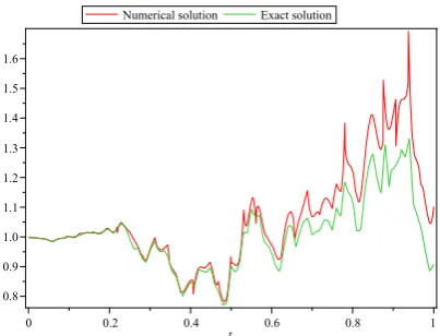
Example 6.1. Consider the following stochastic Itˆo-Volterra integral equation [3, 7]
X(t) = 1 +
Z t
0
s2X(s)ds+
Z t
0
sX(s)dB(s), s, t∈[0,1], (52)
where X(t) is an unknown stochastic process defined on the probability space (Ω,F, P), andB(t) is a Brownian motion process. The exact solution of this stochastic Itˆo-Volterra integral equation is
X(t) = exp
t3 6 +
Z t
0
sdB(s)
. (53)
The stochastic operational matrix of Legendre wavelets and the presented method in section 5 are employed for deriving a numerical solution of this Itˆo-Volterra integral equation. The approximate solution computed by the presented method and exact solution are represented in Fig. 6.1 for mˆ = 128. The absolute error of the numerical results are shown in the Table 6.1 for different values ofm.ˆ
Figure 1. The approximate solution and exact solution for ˆm= 128.
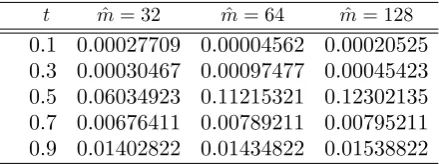
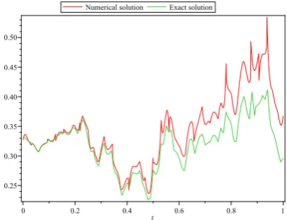
Example 6.2. Let us consider the following stochastic Itˆo-Volterra integral equation [3,7]
X(t) = 1 12 +
Z t
0
cos(s)X(s)ds+
Z t
0
sin(s)X(s)dB(s), s, t∈[0,1], (54)
Table 1. The absolute error of the numerical results for different values of ˆm.
t mˆ = 32 mˆ = 64 mˆ = 128
0.1 0.00319130 0.00057210 0.00222540 0.3 0.00371524 0.00917624 0.00402876 0.5 0.44932060 0.86719460 0.95334270 0.7 0.05396580 0.06228580 0.06238580 0.9 0.12015880 0.12185880 0.13135880
integral equation is
X(t) = 1 12exp
−t
4 + sin(t) +
sin(2t) 8 +
Z t
0
sin(s)dB(s)
. (55)
This stochastic Itˆo-Volterra integral equation is solved by using the stochastic operational matrix of Legendre wavelets and the proposed method in section 5. In Fig. 6.2 the ap-proximate solution computed by the presented method and exact solution are shown for
ˆ
m= 128. The absolute error of the numerical results for different values of mˆ are shown in the Table 6.2.
Figure 2. The approximate solution and exact solution for ˆm= 128.
Table 2. The absolute error of the numerical results for different values of ˆm.
t mˆ = 32 mˆ = 64 mˆ = 128
0.1 0.00027709 0.00004562 0.00020525 0.3 0.00030467 0.00097477 0.00045423 0.5 0.06034923 0.11215321 0.12302135 0.7 0.00676411 0.00789211 0.00795211 0.9 0.01402822 0.01434822 0.01538822
Example 6.3. Consider the following stochastic Itˆo-Volterra integral equation [6]
X(t) = 1 3+
Z t
0
ln(s+ 1)X(s)ds+
Z t
0
p
ln(s+ 1)X(s)dB(s), s, t∈[0,1], (56)
integral equation is
X(t) = 1 3exp
−t
2 + 1
2tln(t+ 1) + 1
2ln(t+ 1) +
Z t
0
p
ln(s+ 1)dB(s)
. (57)
The Legendre wavelets stochastic operational matrix and the proposed method in section 5 are used for solving this stochastic Itˆo-Volterra integral equation. The exact solution and approximate solution computed by the presented method for mˆ = 128 are shown in Fig. 6.3. The absolute error of the numerical results are shown in the Table 6.3 for different values of m.ˆ
Figure 3. The approximate solution and exact solution for ˆm= 128.
Table 3. The absolute error of the numerical results for different values of ˆm.
t mˆ = 32 mˆ = 64 mˆ = 128
0.1 0.00102914 0.00106840 0.00142866 0.3 0.00344068 0.00001788 0.00625188 0.5 0.11389535 0.28145811 0.31242841 0.7 0.03226066 0.03587166 0.03487166 0.9 0.05533170 0.05679170 0.05930170
7. Conclusion
A new stochastic operational matrix for the Legendre wavelets is derived. The BPFs and their relation with Legendre wavelets are used to derive this stochastic operational matrix. An efficient computational method based on this stochastic operational matrix is introduced for solving stochastic Itˆo-Voltera integral equations. Convergence and error analysis of the Legendre wavelets basis are considerd. Efficiency of the proposed method is confirmed by some numerical examples.
References
[1] Kloeden, P. E. and Platen, E., (1992), Numerical Solution of Stochastic Differential Equations, Springer-Verlag. New York.
[3] Maleknejad, K., Khodabin, M. and Rostami, M., (2012), Numerical solution of stochastic Volterra integral equations by a stochastic operational matrix based on block pulse functions. Mathematical and Computer Modelling, 55(3), pp. 791-800.
[4] Maleknejad, K., Khodabin, M. and Rostami, M., (2012), A numerical method for solving m-dimensional stochastic Itˆo-Volterra integral equations by stochastic operational matrix. Computers and Mathematics with Applications, 63(1), pp. 133-143.
[5] Khodabin, M., Maleknojad, K. and Hossoini Shckarabi, F., (2013), Application of triangular func-tions to numerical solution of stochastic Volterra integral equafunc-tions. IAENG International Journal of Applied Mathematics, 43(1), pp. 1-9.
[6] Khodabin, M., Maleknejad, K., Rostami, M. and Nouri, M., (2012), Numerical approach for solving stochastic Volterra-Fredholm integral equations by stochastic operational matrix. Computers and Mathematics with Applications, 64(6), pp. 1903-1913.
[7] Heydari, M. H., Hooshmandasl, M. R., Ghaini, F. M. and Cattani, C., (2014), A computational method for solving stochastic Itˆo-Volterra integral equations based on stochastic operational matrix for generalized hat basis functions. Journal of Computational Physics, 270, pp. 402-415.
[8] Cortes, J. C., Jodar, L. and Villafuerte, L., (2007), Numerical solution of random differential equations: a mean square approach. Mathematical and Computer Modelling, 45(7), pp. 757-765.
[9] Cortes, J. C., Jodar, L. and Villafuerte, L., (2007), Mean square numerical solution of random differ-ential equations: Facts and possibilities. Computers and Mathematics with Applications, 53(7), pp. 1098-1106.
[10] Jankovic, S. and Ilic, D., (2010), One linear analytic approximation for stochastic integrodifferential equations. Acta Mathematica Scientia, 30(4), pp. 1073-1085.
[11] Strang, G., (1989), Wavelets and dilation equations: A brief introduction. SIAM review, 31(4), pp. 614-627.
[12] Boggess, A. and Narcowich, F. J., (2009), A first course in wavelets with Fourier analysis. John Wiley and Sons.
[13] Razzaghi, M. and Yousefi, S., (2001), The Legendre wavelets operational matrix of integration. Inter-national Journal of Systems Science, 32(4), pp. 495-502.
[14] Razzaghi, M. and Yousefi, S., (2000), Legendre wavelets direct method for variational problems. Mathematics and Computers in Simulation, 53(3), pp. 185-192.
[15] Mohammadi, F., Hosseini, M. M. and Mohyud-Din, S. T., (2011), Legendre wavelet galerkin method for solving ordinary differential equations with non-analytic solution. International Journal of Systems Science, 42(4), pp. 579-585.
[16] Mohammadi, F. and Hosseini, M. M., (2011), A new Legendre wavelet operational matrix of derivative and its applications in solving the singular ordinary differential equations. Journal of the Franklin Institute, 348(8), pp. 1787-1796.
[17] Jiang, Z., Schoufelberger, W., Thoma, M. and Wyner, A., (1992), Block pulse functions and their applications in control systems. Springer-Verlag New York, Inc.
[18] Liu, N. and Lin, E. B., (2010), Legendre wavelet method for numerical solutions of partial differential equations. Numerical Methods for Partial Differential Equations, 26(1), pp. 81-94.