Volume 3, 2018, Pages 1324–1331
HIC 2018. 13th International Conference on Hydroinformatics
Towards Transient Experimental Water Surfaces:
Strengthening Two-Dimensional SW Model Validation
Mart´ınez-Aranda, S.
1,∗, Fern´
andez-Pato, J.
1,2, Caviedes-Voulli`
eme, D.
3,
Garc´ıa-Palac´ın, I.
1, and Garc´ıa-Navarro, P.
11 LIFTEC-CSIC, University of Zaragoza, Spain 2
Hydronia Europe SL, Madrid, Spain
3 Chair of Hydrology, Brandenburg University of Technology, Cottbus, Germany
Abstract
The measurement and simulation of 2D free-surface shallow flows is carried out in this work. For the experimental study a 3D-sensing device (Microsoft Kinect) is used to measure both steady and transient water surface elevation fields with different flow characteristics. This procedure provides 640x480 px resolution water surface level point clouds with a frequency ranging from 8 Hz to 30 Hz. The experimental measurements are compared with 2D finite volume simulations carried out by means of a robust and well-balanced numerical scheme able to deal with flow regime transitions and wet/dry fronts. A good agreement is found between experimental and numerical results for all the cases studied, demonstrating the capability of the RGB-D sensor to capture the water free-surface position accurately. This new experimental technique, which allows us to obtain 2D water depth fields in open-channel flows, leads to a wide range of promising capabilities in order to validate new shallow water models and to improve their accuracy and performance.
1
Introduction
Shallow water solvers have received wide attention in the past decade, resulting in a new generation of robust, efficient and accurate models [5] which currently allow for large scale and long term computations of complex transients on both natural and man-made environments. These new solvers have been systematically verified against 1D and 2D analytical solutions for simplified problems [7, 8]. In addition, they have also been validated using laboratory experiments [4,10], as well as some well-documented real-scale field cases [6,3]. Despite the 2D nature of the aforementioned benchmark tests, none of them reports 2D transient water surface elevations. The nonavailability of laboratory 2D transient water surface data is due to the technical difficulties in measuring a fast moving water surface. Furthermore, in experimental fluid mechanics, measuring the evolution of a free surface has received little attention.
As numerical models have become more sophisticated, more complex flow phenomena can be, in principle, accurately simulated. Perhaps some of the most challenging ones are fast
sensors, is clearly their very affordable cost, which makes them an attractive tool for many researchers, despite their limitations. A few pioneering studies have been reported in Hydraulic or Fluid Mechanics applications of RGB-D sensors. A proof-of-concept experiment was car-ried out in [2] to demonstrate the feasibility of capturing moving opaque water surfaces with a Kinect device. The transient dynamics of a fast-moving granular surface was measured in [1] with a Carmine device. Recently, [9] observed surface water gravity waves in clear water in a flume, as a proof-of-concept that refraction can be used for such purposes.
In this work, we present a set of 2D transient shallow water experiments in a laboratory flume involving steady transcritical flows and dam-break cases. In all cases we report the 2D temporal evolution of the water surface captured by means of a commercial-grade RGB-D device measuring opaque water. The aim of the study is to demonstrate that this technique can be used to generate new benchmark tests for the current and future generations of 2D shallow water models, both to validate their capabilities and identify the next set of challenges to be solved. We also point out that this is the first application –to the authors knowledge– of RGB-D sensors for the measurement of complex transient shallow water dynamics.
2
Experimental setup
The experiments were performed on a 6 m long rectangular cross-section (240x150 mm) plex-igass flume of approximately zero slope (0.00092 m/m) along a 3.26 m length reach, followed by a kink to a slope of 0.0404 m/m to force supercritical flow downstream (Figure 1). A pneumatically-actuated gate separated the flume from an upstream reservoir and generated dam-break conditions with different water elevations. Furthermore, a closed circuit allowed to establish steady flow in the flume. The downstream flume boundary was always an outfall into a recirculation tank. Different elements were employed to reproduce some interesting phe-nomena in the free-surface flow. In this work a simple geometry was constructed by placing a rectangular obstacle (16.3x8.0x7.0 cm) at the center of the flume and 2.05 m downstream the gate. The obstacle was constructed out of PVC. Manning’s roughness coefficient for the plexiglass flume and the PVC obstacle was estimated as 0.01 sm-1/3.
Measurements of the free-surface position were recorded using a consumer-grade RGB-D sensor Microsoft Kinect (Microsoft, 2010). The device was suspended 0.7 m above the flume floor, ensuring an optimal compromise between field-of view, 2D resolution level and depth-accuracy for the measured depth data. In transient flow measurements, the dam-break initial time was captured by placing an indicator LED light on the flume structure within the field-of-view of the RGB-D sensor. This LED was lighted while the gate actuated, allowing to register the initial time for the transient flow and the duration of gate-opening (Figure2).
Figure 1: Experimental setup: flume geometry.
by the object shape. The deformed pattern is recorded by a monochrome NIR camera from a different position and depth information can be extracted from the disparity from the original projected pattern. In these experiments, instantaneous 2D free-surface position fields were captured with random time steps, ranging from 30 (30 fps) and 125 (8 fps) milliseconds and depending that on the sensor capability.
Figure 2: Experimental setup: RGB-D sensor scheme.
Fuerthermore, the SL pattern projected by the RGB-D sensor needs to be reflected by the free-surface in order to observe it. The transparent nature of water does not allow for this. A simple solution is to tint water until it becomes opaque and reflects the pattern at the surface [2]. We tinted the water with titanium oxide (TiO2) at a concentration of 1.2% in mass. This allowed to reflect the pattern off the water surface, thus not requiring reflection corrections as proposed by [9]. In addition to the transient flow surfaces, the flume bed and obstacles were also previously captured with the RGB-D sensor in a dry condition, to completely characterize the experimental geometry within the device field-of-view.
3
Governing equations and numerical model
In this work, the free surface flow is modelled by means of the 2D SWE that can be expressed as follows: ∂h ∂t + ∂qx ∂x + ∂qy
∂y = 0 (1)
∂qx ∂t + ∂ ∂x q2 x h + 1 2gh 2 + ∂ ∂y
qxqy h
=gh(S0x−Sf x) (2)
∂qy
∂t + ∂ ∂x
qxqy h + ∂ ∂y q2 y h + 1 2gh 2 !
=gh(S0y−Sf y) (3)
where hrepresents the water depth, (qx, qy) the depth-averaged components of the discharge
vector along the (x, y) coordinates, (S0x, S0y) the slope term components and (Sf x, Sf y) the
friction-associated losses.
The system of equations is numerically solved by means of a robust and well-balanced upwind (FOU) scheme, in the frame of finite volume methods family. As the method uses an explicit time discretization, the time step is restricted due to stability issues. For this reason, a GPU-based implementation is used in order to reduce the computational effort. This numerical scheme has been widely and successfully tested and it is chosen to validate the 3D sensing measuring technique. For numerical simulation of the experimental cases tested in laboratory, the domain is discretized by means of an unstructured triangular mesh with 50000 cells, refined at the obstacle position.
4
Comparison of experimental and numerical results
4.1
Steady flow
A constant inlet dischargeQ= 9.02m3/hwas set at the flume and the flow was developed until it reached the steady state. The flow regime was subcritical upstream the rectangular obstacle and evolved to supercritical downstream. A complex wave structure was created by reflection at both the flume walls and the centered object, leading to a diamond shape wake downstream the obstacle. Figure3 shows the 2D steady water depth fields from laboratory measurements and numerical simulation. The experimental RGB-D sensor data agree properly with the flow structure predicted by the numerical model, almost showing a similar wave position and water depth values.
Figure 3: Experimental (left) and numerical (right) 2D water depth fields for the steady case.
depth gradient isolines. The more marked differences were found at both sides of the centered obstacle, where the oblique shock wave predicted by the computational model appeared down-stream for the Kinect measurements. Nevertheless, the RGB-D sensor demonstrated to be able to capture properly a complex free-surface structured, regardless of the temporal fluctuations caused by turbulence.
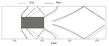
Figure 4: Wave structure comparison: experimental (dashed lines) and numerical (solid lines).
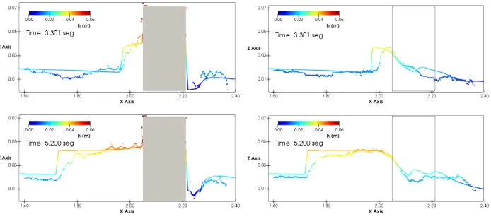
Water depth profile along the flume central line (top row) and cross-section profiles at x = 2.08 m (bottom row left) and x = 2.30 m (bottom row right) are displayed in Figure
5. Comparison of numerical and laboratory results show a suitable agreement. The highest differences appeared at the obstacle wake, where the RGB-D sensor measured a narrower shape than that predicted by the numerical model.
interest until it reached the centered obstacle att≈2.6s. A shock wave appeared immediately at the front of the obstacle, increasing its water depth with time and taking a curved shape (t = 3.051 s). Downstream, water finally surrounded the obstacle and a narrow diamond wake was formed (t = 3.301 s). The frontal shock wave developed to a hydraulic jump fully perpendicular to the main flow direction (t = 3.863 s), which moved upstream until it was dissipated at the boundary reservoir.
(Continue in the next page.)
Figure 6: Temporal evolution of the experimental (left column) and numerical (right column) 2D water depth fields for the dam-break case.
the shock wave appearance step. Moreover, the lateral and wake flow structure was also well captured by the Kinect, demonstrating the ability of the experimental technique to handle fast free-surfaces movements with small water depths.
Finally, one of the most interesting features that this new experimental technique offers is the capability to extract the water depth temporal evolution along any longitudinal or cross-direction profile, and not only in points where a pressure gauge was placed. That becomes a versatile tool which allows us to study the flow evolution in profiles not previously set up at laboratory. Figure7depicts the water depth temporal evolution along both the flume axis (Y = 12cm) and the longitudinal profile centered at the flume wall-obstacle gap (Y = 20cm). The experimental profiles obtained from the Kinect data showed a correct agreement with the numerical water depth profiles.
required laboratory setup is inexpensive and offers a simple implementation in comparison with existing experimental techniques. Instantaneous two-dimensional water depth fields were obtained for dam-break and steady flows and were compared with finite volume simulations carried out by means of a robust and well-balance numerical scheme. Results show that this new technique allows us to generate new benchmark tests for the current and future generations of 2D shallow water models.
6
Acknowledgments
This work was partially funded by the MINECO/FEDER under research project CGL2015-66114-R and by Diputacion General de Aragon, DGA, through Fondo Europeo de Desarrollo Regional, FEDER. The experimental data set is available inhttp://fiona.cps.unizar.es/
~ghcuser/Kinect_exp_data.zip
References
[1] D. Caviedes-Voulli`eme, C. Juez, J. Murillo, and P. Garc´ıa-Navarro. 2D dry granular free-surface flow over complex topography with obstacles. Part I: experimental study using a consumer-grade RGB-D sensor. Computers & Geosciences, 73:177–197, 2014.
[2] B. Combes, A. Guibert, E. M´emin, and D. Heitz. Free-surface flows from kinect: Feasibility and limits. InProceedings of FVR-2011, Poitiers, France, 2011.
[3] J. Fern´andez-Pato, D. Caviedes-Voulli`eme, and P. Garc´ıa-Navarro. Rainfall/runoff simulation with 2d full shallow water equations: Sensitivity analysis and calibration of infiltration parameters.
Journal of Hydrology, 536:496–513, 2016.
[4] L. Fraccarollo and E.F. Toro. Experimental and numerical assessment of the shallow water model for two-dimensional dam-break type problems. Journal of Hydraulic Research, 33(6):843–658, 1995.
[5] P. Garc´ıa-Navarro. Advances in numerical modelling of hydrodynamics workshop. InApplied Mathematical Modelling, volume 40, page 7423, University of Sheffield, UK, 2016.
[6] J.M. Hervouet and A. Petitjean. Malpasset dam-break revisited with two-dimensional computa-tions. Journal of Hydraulic Research, 37(6):777–788, 1999.
[7] I. MacDonald, M.J. Baines, N.K. Nichols, and P.G. Samuels. Analytic benchmark solutions for open-channel flows. Journal of Hydraulic Engineering, 123(11):1041–1045, 1997.
[8] J. Murillo and P. Garc´ıa-Navarro. Augmented versions of the hll and hllc riemann solvers including source terms in one and two dimensions for shallow flow applications. Journal of Computational Physics, 231(20):6861–6904, 2012.
[9] A. Nichols and M. Rubinato. Remote sensing of environmental processes via low-cost 3D free-surface mapping.Computers & Geosciences, 73:177–197, 2016.