Studies on Structure and Property of Polymer-based Nano-composite Materials

(1)

University of New Orleans University of New Orleans

ScholarWorks@UNO

University of New Orleans Theses and

Dissertations Dissertations and Theses

Spring 5-17-2013

Studies on Structure and Property of Polymer-based

Nano-composite Materials

composite Materials

Yun Zhai

[email protected]

Follow this and additional works at: https://scholarworks.uno.edu/td

Part of the Materials Science and Engineering Commons, and the Mechanical Engineering Commons

Recommended Citation Recommended Citation

Zhai, Yun, "Studies on Structure and Property of Polymer-based Nano-composite Materials" (2013). University of New Orleans Theses and Dissertations. 1680.

https://scholarworks.uno.edu/td/1680

This Dissertation is protected by copyright and/or related rights. It has been brought to you by ScholarWorks@UNO with permission from the rights-holder(s). You are free to use this Dissertation in any way that is permitted by the copyright and related rights legislation that applies to your use. For other uses you need to obtain permission from the rights-holder(s) directly, unless additional rights are indicated by a Creative Commons license in the record and/ or on the work itself.

(2)

Studies on Structure and Property of Polymer-based

Nano-composite Materials

A Dissertation

Submitted to the Graduate Faculty of the University of New Orleans

in partial fulfillment of the requirements for the degree of

Doctor of Philosophy in

Engineering and Applied Science Mechanical Engineering

by

Yun Zhai

B.S. Southwest JiaoTong University, Chenddu, China, 2006 M.S. Southwest JiaoTong University, Chengdu, China, 2008

(3)

ii

DEDICATION

(4)

iii

ACKNOWLEDGEMENT

First of all, I would like to show my thankfulness to my chief advisor Prof. David

Hui for the opportunity to work with him on this promising project. Discussions with

Prof. Hui always enlightened me a lot and helped to save me large amount of time on the

experiment design. I would also like to thank Prof. Hui for offering me opportunity to

travel to other research center and collecting valuable data from advanced facilities. His

patience with me, guidance for my research and wise suggestion will always be deeply

appreciated.

I would like to thank Dr. Kazim Akyuzlu, Dr. Weilie Zhou, Dr. Huimin Chen, and

Dr. Hall Carsie for serving on my committee.

Acknowledgements are also due to the Defense Advanced Research Projects

Agency for their financial support and Advanced Materials Research Institute at

University of New Orleans for their advanced facilities and resources.

I am thankful to Dr. Kazim M. Akyuzlu, Dr. Dongming Wei, Dr. Carsie A. Hall,

Dr. Weilie Zhou, Dr. Salvadore Guccione, Dr. Kenneth Holladay for all they have taught

me and all the help they offered. Special thanks to Dr. Weilie Zhou’s PhD student Kai

Wang and postdoctoral Dr. Baobao Cao for the assistance on the training of scanning

electron microscope and transmission electron microscopy.

I would also like to express my gratitude towards Prof. Mircea Chipara,

University of Texas Pan American, for his advices, patience, and gentleness during my

(5)

iv

experimental data interpretation. I also want to thank Prof. Chipara for the assistance on

Raman spectroscopy characterization which helped me to identify the carbon nanotube

feature in the composite materials.

Finally, I would like to thank my family for their unconditional love. Their

(6)

v

ABSTRACT

The mixing of polymers and nanoparticles makes it possible to give advantageous

macroscopic material performance by tailoring the microstructure of composites. In this

thesis, five combinations of nano inclusion and polymer matrix have been investigated.

The first type of composites is titanium dioxide/ polyaniline combination. The

effects of 4 different doping-acids on the microstructure, morphology, thermal stability

and thermoelectric properties were discussed, showing that the sample with HCl and

sulfosalicylic dual acids gave a better thermoelectric property. The second combination is

titanium dioxide/polystyrene composite. Avrami equation was used to investigate the

crystallization process. The best fit of the mass derivative dependence on temperature has

been obtained using the double Gaussian dependence. The third combination is titanium

dioxide/polyaniline/ polystyrene. In the titanium dioxide/polyaniline/ polystyrene ternary

system, polystyrene provides the mechanical strength supporting the whole structure;

TiO2 nanoparticles are the thermoelectric component; Polyaniline (PANI) gives the

additional boost to the electrical conductivity. We also did some investigations on

Polyethylene odide-TiO2 composite. The cubic anatase TiO2 with an average size of

13nm was mixed with Polyethylene-oxide using Nano Debee equipment from BEE

international;

Single wall carbon nanotubes were introduced into the vinyl acetate-ethylene

copolymer (VAE) to form a connecting network, using high pressure homogenizer (HPH).

(10)

ix

sample quality. Theoretical percolation was derived according to the excluded volume

theory, turning out the threshold () as a function of aspect ratio (A) to be

1 exp .

Key words: Single wall carbon nanotube, polymer, titanium dioxide, thermoelectric,

(11)

1

CHAPTER 1 LITERATURE REVIEW

1.1. Introduction and Background

Polymer composites have broad applications in industry products, such as

sporting goods, aerospace components, automobile, because the composite material

combines the excellent physical properties of the Nano filler and the mechanical stability

of the polymer matrix. The clay-reinforced resin was introduced in the early 1900’s as

one of the first mass-produced polymer-nanoparticle composites[1]. In early 1990s,

Toyota researchers revealed the introduction of mica into nylon produced a five-fold

increase in the yield and tensile strength of the material[2]. After that, the

polymer-nanoparticle composites became a popular research area in material science and

engineering. The final products do not have to be in nanoscale, but can be micro- or

macroscopic in size. This surge in the field of nanotechnology has been greatly facilitated

by the application of scanning tunneling microscopy and scanning probe microscopy in

the early 1980s[3]. Also the increasing application of computer modeling and simulation

has made it easier to design and predict the material performance at the nanoscale[4].

The material physical properties changes significantly when micro particles

transits to nanoparticles. One main character of nanoscale materials is the large surface

for a given volume. When the particle size transits from micro to nanoscale, the physical

properties changes dramatically because many chemical and physical interaction are

(12)

2

Figure 1.1 is the common particle geometries and their surface area-to–volume ratios. The area-to-volume ratios are dominated by the first term in the equation

especially for the fiber and layered material. The second term (2/l and 4/l) is often

omitted compared to the first term. Therefore when the particle diameter, layer thickness

and fibrous material diameter change from micrometer to nanometer, the surface

area-to-volume ratio will be affected by three orders of magnitude[5].

(13)

3

1.2. Layered Nano-Inclusion and Polymer Matrix

According to interaction between the nano layer and polymer matrix, three types

of nanocomposites can be defined. We use layered silicate and polymer composite as

example[6].

If no polymers get involved into the interspace between silicate layers, as shown

in Figure 1.2(a), the layers exist as a separated phase in the matrix. This is so-called

phase separated nanocomposite. The layered phase can be identified by X-Ray diffraction,

Figure 1.3(a)[7]. When the polymer chain is intercalated between the silicate layers, it

becomes intercalated nanocomposite. Since the interspaces between the layers are

increased, the peak of layer phase shifts towards the lower angle values, Figure 1.3(b). If

the nano layers are dispersed well enough with spacing larger than 8nm, the layer phase

(14)

4

(15)

5

(16)

6

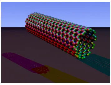
1.3. Structure of Single Wall Carbon Nanotube

Single wall carbon nanotube is a single layer of a graphite crystal rolled up into a

seamless cylinder. The cylinder wall is 1 atom thick and the tube has 10-40 numbers of

carbon atoms along the circumference and a micron scale length along the cylinder axis[8]

(Figure 1.4).

Figure 1.4 Single wall carbon nanotube

Each SWNT is specified by the chiral vectorC, which is often described by the

pair of indices n, m that denote the number of unit vector naand ma in the hexagonal

honeycomb lattice.

(17)

7

The physical meaning of chiral vector is the description of how graphite sheet is

rolled up. The chiral angle θ is the angle between the unite vector a and chiral vectorC,

as showed in Figure 1.5. Three types of single wall carbon nanotube can be defined

according to the chiral angle. When θ =0°, it is called zigzag nanotube; when θ =30°, it’s

called armchair nanotube; when 0° ! 30° , it’s called chiral nanotube. The

translation vector T is perpendicular to the chiral vectorC, meaning the axial direction of

the nanotube cylinder and therefore the length of vector |C| can be understood as

circumference of bottom plane.

(18)

8

1.4. Electronic Properties of Nanotubes

In the field of material science, microstructure determines the physical properties

of material. As for carbon nanotube, the electronic property mainly depends on two

structure factors: the chirality and the diameter. As we mentioned before, the chirality of

carbon nanotube can be described by a pair of indicesn, m. When n m(armchair), the

nanotubes show metallic properties; When n m 3p, where p is an integer, the

nanotubes are expected to show metallic property; When n m $ 3p, the nanotubes are

expected to semi-conducting materials[10]. Figure 1.6 shows the conducting properties

with respect to chiralities on a 2-dimensional graphite sheet.

(19)

When it comes to diameter, the band gap theory needs to be considered. As

showed in Figure 1.7, the higher band gap energy

valence band, the lower conductivities of the material.

Figure 1.7 The electronic band structure of metals, semiconductors, and insulators

The band gap can be

where is the C-C tight-binding overlap

distance in graphite sheet;

see the band gap energy is inversely proportional to

Jeroen W. G et al experimentally showed the value of

diameter ranging from 0.6 to 1.1nm

9

it comes to diameter, the band gap theory needs to be considered. As

, the higher band gap energy between the conduction band

valence band, the lower conductivities of the material.

he electronic band structure of metals, semiconductors, and insulators

can be described as

binding overlap energy; is the nearest neighbor

is the diameter of the nanotube. From this equation we can

is inversely proportional to the diameter of the nanotube.

et al experimentally showed the value of as a function

diameter ranging from 0.6 to 1.1nm[11], as showed in Figure 1.8.

it comes to diameter, the band gap theory needs to be considered. As

the conduction band and the

he electronic band structure of metals, semiconductors, and insulators

(1.2)

neighbor C-C

is the diameter of the nanotube. From this equation we can

the diameter of the nanotube. Wilder,

(20)

10

(21)

11

1.5. Mechanical Properties of Carbon Nanotubes

Since the discovery of carbon nanotube[12-15], it was expected to display similar

stiffness like graphite with in-plane modulus of 1.06TPa[16]. An empirical lattice

dynamics model was used to predict the elastic properties of single and multilayered

nanotubes[17], Figure 1.9. JP Lu concluded that elastic moduli are insensitive to size and

helicity and the Young's and shear moduli of nanotubes are comparable to that of

diamond.

(22)

12

Wong et al made a direct measurement on elasticity, strength and toughness of

multi wall nanotubes[18]. They used AFM to measure the bending force versus

displacement along the unpinned lengths of nanotube, Figure 1.10. After the AFM tip

made contact with nanobeam, the measured lateral force increased linearly as the

nanobeam was elastically displaced from its equilibrium position.

Figure 1.10 AFM tip scanning perpendicular to the axis of the nanobeam[18]

A typical F d data was acquired to determine the E of a nanotube. According to

the F d curve, force constant as a function of position was obtained, Figure 1.11, where

force constant kx ()

(* .They got the average E value of 1.28 . 0.59TPa with no

dependence on tube diameter, similar to the in-plane modulus of graphite 1.06TPa. The

(23)

13

(24)

14

1.6. Application of Atomic Force Microscope

Atomic force microscope was invented by Binning, Quate and Gerber in 1986[19].

It is a powerful tool to detect the material surface topography in nano scale. Figure 1.12 is

the central component of the AFM system used in this research. The major parts from top

to bottom are laser head, probe holder and probe, scanner, motor control and base. The

height value as a function of position x, y is collected when a sharp probe is scanned

across the material surface.

(25)

15

The laser path is showed in Figure 1.13. A laser is generated from the laser head 1

and then reflected by the mirror 2, hit the back of cantilever, reflected by the tilt mirror 4

and finally detected by the photodetector 5.

Figure 1.13 Multimode AFM laser head

There 2 typed of scanning method for this AMF: contact mode and tapping mode.

Contact mode AFM operates by scanning a tip attached to the end of a cantilever across

the sample surface while monitoring the change in cantilever deflection with a split

photodiode detector. A feedback loop, Figure 1.14(a), maintains a constant deflection

between the cantilever and the sample by vertically moving the scanner at each x, y

data point to maintain a “setpoint” deflection. By maintaining a constant cantilever

(26)

16

Tapping Mode AFM operates by scanning a tip attached to the end of an

oscillating cantilever across the sample surface. The cantilever is oscillated at or slightly

below its resonance frequency with amplitude ranging typically from 20nm to 100nm.

The tip lightly “taps” on the sample surface during scanning, contacting the surface at the

bottom of its swing. The feedback loop, Figure 1.14(b), maintains a constant oscillation

amplitude by maintaining a constant RMS of the oscillation signal acquired by the split

photodiode detector.

Figure 1.14 (a) contact mode (b) tapping mode

Atomic Force microscope can be used to detect interfacial adhesion between the

nanotube and surrounding polymer[20]. One end of nanotube is attached on the tip of

AFM and the other end is embedded in polymer matrix. During the polling out process,

the interfacial shear strength can be measured by detecting the cantilever bending force,

as showed in Figure 1.15. Increasing the nanotube embedded length causes the nanotube

to break instead of pullout from the polymer. As a result, the forces required to pull out

(27)

17

(28)

18

Figure 1.16 The force required to pull out nanotubes embedded at various lengths[20]

Atomic force microscopy-based nanoindentation can be used to map the nano

scale mechanical properties like elasticity and stiffness. Dusan Losic et al performed

nanoindentation on cribellum surface using Veeco Dimension 3000 AFM with diamond

tip[21], Figure 1.17. Typical force penetration curve with loading and unloading can also

(29)

19

(30)

20

1.7. Raman Spectroscopy

When a strain is applied to a nano composite material, the interatomic distances of

C-C change, and thus the vibrational frequencies of some of the normal modes change

causing a Raman peak shift.

The Raman spectrum for nanotubes has been well documented by Rao, A. M et

al[22]. They did lattice dynamics calculations based on C-C force constant. The

intensities and frequencies turned out to agree well with Raman scattering measurement,

Figure 1.18.

(31)

21

C.A. Cooper et al observed that G5 Raman band shifts to a higher wavenumber

when the SWCTs is under hydrostatic pressure, Figure 1.19; while G5 Raman band shifts

to a lower wavenumber when tensile stress is applied, Figure 1.20[23]. They

demonstrated that the effective modulus of SWNTs dispersed in a composite could be

over 1 TPa.

(32)

22

Figure 1.20 Variation of the 65 Raman peak position with tensile strain for pulsed laser SWNT dispersed in epoxy resin[23].

Schadler, L. St al found the second order band of multiwall carbon nanotube

shifts slightly positive in tension and negatively in compression, Figure 1.21[24]. The

large shift in compression compared to tension indicates that the MWCTs carry more

(33)

23

.

(34)

24

1.8. Dispersion of Nanotube in Polymer

It is quite a challenge to achieve a high degree dispersion of SWNTs in polymer

matrix due to their tendency to aggregate in bundles and agglomeration[25]. Wise, K.E et

al dispersed SWNTs in a nitrile functionalized polyimide matrix[26]. They observed G

band upshifts in Raman spectra which indicate a noncovalenet interaction between

nanotube and polymer, Figure 1.22.

(35)

25

Badaire, Stéphane et al measured the dimentions of CNTs in dispersed state via

Depolarized dynamic light scattering[27]. They studied the effect of sonication time and

power on the dispersion of nanotube in surfactant solutions, as showed in Table 1.1. The

diameter of the SWNT bundles decrease with the incraeasing of sonication time at a

constant pressure.

Table 1.1 Influence of Sonication Time and Power on the Dimensions of CNT Bundles[27]

Barry J. Bauer et al used small angle neutron scattering to determine the average

dispersion of large collection of SWNTs. They applied power law to measure the degree

of aggregation[28]. For example, a slope of between -2 and -3 for a chain molecule such

as polymer or a SWNT strongly suggests aggregation, Figure 1.23 Power law scattering

(36)

26

Figure 1.23 Power law scattering from fractal objects[28]

Dale W. Schaefer et al used small angle X-ray scattering to determine the

morphology of carbon nanotube suspension on a scale of 1nm-50µm[29]. They found the

morphology is dominated by a network structure of aggregated tubes instead of rod like

(37)

27

1.9. Fabrication of Nanotube/Polymer Composite

Three mainly fabrication methods have been used to synthesize nanotube/polymer

composite: solution blending, melt blending and in situ polymerization. All methods are

to improve the nanotube dispersion in polymer matrix because a homogeneous

distribution of nanotube has a great influence on composite performance[30].

1.9.1 Solution Blending

The solution blending is the most popular method to fabricate the

nano-composite[31]. Three major steps are involved in solution blending: disperse nanotubes

in a solvent; mix the solvent with polymer which can be solid or emulsion; drying the

solution into a solid composite. Before the drying process, usually a high power

sonication is applied to make a temperately suspension with nanotube[32]. It is common

for researchers to use different kinds of surfactants to modify the surface of the nanotube

and make the tubes stable in the solution[33].

M. F. Islam et al used NaDDBS(C12H25C6H4SO3Na) as surfactant to exfoliate

nanotube bundles into single tubes with a fraction of 63±5% in water[32]. They used

tapping mode AFM to measure the fraction of single tubes. The tube diameters were

derived from height measurements. As showed in Figure 1.24, the shaded regions define

(38)

28

Figure 1.24 Length and diameter distribution of HiPCO tubes dispersed by the bath sonicator[32]

Xiaoyi Gong et al used Polyoxyethylene 8 lauryl as nonionic surfactant to

dissolve nanotube in acetone with mechanical stirring[34]. The addition of 1 wt % carbon

nanotubes in the composite increases the glass transition temperature from 63 °C to 88 °C.

As shown in Figure 1.25(b), the agglomerated carbon nanotubes without surfactant can

(39)

29

Figure 1.25 SEM photographs of carbon nanotubes on fracture surfaces of the composite samples: (a) with surfactant and (b) without surfactant[34]

1.9.2 Melt Blending

Melt processing method is suitable to deal with thermoplastic polymers which can

be easily softened when heated. When the heating temperature is above the polymer glass

transitionT₇, semi-crystalline polymers become soft enough to form a viscous liquid[35].

(40)

30

form of compression molding, injection molding or extrusion[36]. Several groups have

report their composite samples processed by melt blending in Polystyrene[37],

PMMA[38], polypropylene[39], PBO[40].

R. Haggenmueller et al combined the solvent casting and melt mixing to disperse

SWNT in PMMA[38]. They broke solvent casting film into pieces and hot pressed the

pieces at 1808 and 3000lb for 3 minutes. The melt mixing procedure was repeated up to

(41)

31

Figure 1.26 Optical micrographs of a SWNT±PMMA nanocomposite (a)solvent casting sample. (b) hot pressing (180°C, 3000 lb, 3 min) for 1 cycle; (c) 5 cycles; (d)

20 cycles[38].

Emilie J. Siochi et al used melt extrusion and fiber drawing process to align

SWNT in the fiber direction and achieved higher tensile moduli and yield stress[41].

Figure 1.27 show the single screw extruder developed at NASA Langley Research Center.

A filter (component 4 in the figure) was used in the nozzle to help breaking up

(42)

32

Figure 1.27 Components of extruder used for melt processing of SWCNT/Ultem nanocomposites[41].

Arup R. Bhattacharyya et al[42] mixed polypropylene with 1wt% SWNT in a

Haake rheomix mixer at 2408 at 50rpm for 30min and passed the PP/SWNT composite

through a 300, 250, 120 and 80 mesh filters at 2408. X-ray diffraction was obtained to

(43)

33

Figure 1.28 Integrated wide angle X-ray diffraction intensity of PP/SWNT

composite fiber[42].

1.9.3 In Situ Polymerization

In situ polymerization applies condensation reactions to connect functionalized

nanotubes to the polymer matrix by covalent bonding[43]. The Chemical modification

and functionalization of nanotube can enhance the interaction between pristine nanotubes

and surrounding matrix. If the interfacial bonding is not strong enough, the load transfer

from polymer to nanotube could be limited[44]. Also the sliding of the SWNTs within

the blending of bundles limits the mechanical enhancement due to the disorder of the

(44)

34

Jiang Zhu et al used optimized acid treatment and subsequent fluorination to

disperse functionalized SWNTs into an epoxy composite, increasing 30% in modulus and

18% in tensile strength[47]. Xiaoyi Gong et al reported the introduction of surfactant as

processing aid increased the glass transition temperature from 638 to 888. The elastic

modulus was also increased by more than 30%[34]. Mohammad Moniruzzaman et al

applied high shear mixing of the epoxy resin and SWNT and heat treating the mixture

prior to introducing the hardener to prepare SWNT/epoxy nanocomposites. The whole

method is showed in Figure 1.29. They researched an improvement of 17% in flexural

modulus and 10% in flexural strength at 0.05wt% of nanotubes[48].

(45)

35

1.10. Application of Carbon Nanotube Composites

It has been reported that the tensile modulus and strength of the nanotubes range

about 270Gpa to 1TPa and 11-200GPa [49, 50]. The carbon nanotubes exhibit excellent

tensile strength compared with graphite, Kevlar fibres and stainless steel, as showed in

Figure 1.30[10]. Since the carbon-carbon covalent bonds are one of the strongest in

nature, the tube structure based on such bonds would produce an extraordinary strong

material along the axis of tube. The nanotubes are 100 times stronger than steel but only

one-sixth as heavy as steel making it enable to be used as reinforcements in high strength,

light weight, high performance composites.

(46)

36

CHAPTER 2 TITANIUM DIOXIDE AND POLYANILINE

COMPOSITE

2.1 Thermoelectric Effect and Applications

The thermoelectric effect is the direct conversion of temperature differences to

electric voltage and vice-versa. An applied temperature gradient can cause charge carriers

in the material to diffuse from the hot side to the cold side. Conventional metal or metal

alloys can generate tens of microvolts per degree temperature difference. They are used

in the measurement of temperature or as sensors to operate control systems. However, the

modern semiconductors with material properties and geometry specifically tailored

possess Seebeck coefficients of hundreds of microvolts per degree. The term

“thermoelectric effect” encompassed three separately identified effects: the Seebeck

effect, Peltier effect and Thomson effect.

2.1.1 Seebeck Effect

The Seebeck effect is the conversion of temperature differences directly into

electricity. The thermoelectric energy conversion can be discussed in with reference to

the schematic of a thermocouple shown in Figure 2.1. A and B are two thermoelecments electronically connected. The junctions of A and B are maintained at different

(47)

where and are the thermopowers of material A and B as a function of temperature.

For a small temperature differences the relation is linear, the above formula can be

approximated as:

Figure 2.1 Schematic basic thermocouple. A and B are two different materials.

37

are the thermopowers of material A and B as a function of temperature.

or a small temperature differences the relation is linear, the above formula can be

Schematic basic thermocouple. A and B are two different materials.

are the thermopowers of material A and B as a function of temperature.

or a small temperature differences the relation is linear, the above formula can be

(48)

38

2.1.2 Peltier Effect

In Figure 2.1, if the reverse situation is considered with an external V voltage

applied and a current I flows around the circuit then a rate of heating q occurs at one

junction between A and B and a rate of cooling q occurs at the other. The ratio of I to q

defines the Peltier coefficient Π >

? , representing how much hear current is carried per

unit charge through a given material.

2.1.3 Thomson Effect

The Thomson effect describes the heating or cooling of a current-carrying

conductor with a temperature gradient. If a current density J is passed through a

homogeneous conductor, and there is a temperature difference between two points of the

conductor, the material will either absorb or release heat. The rate of the generation of

heat q per unit volume is:

q ρJ_µJdT

dx

where ρ is the resistivity of the conductor, µ is the Thomson coefficient. The first

term is the Joule heating, the second term is the Thomson heating following J sign

(49)

39

2.1.4 Application of Thermoelectric Devices

Thermoelectric devices are simple and have no moving parts. As shown in the

Figure 2.2 left, when an external power is applied on the thermal couple, negatively

charged electrons carry electrical current in the n-type leg, and positively charged holes

carry the current in the p-type leg. Both the electrons and the holes carry heat away from

the cold side, resulting cooling. Inversely, if a heat source is applied on one side of the

device, as shown in Figure 2.2 right, a voltage can develop on the other side, converting

heat energy to electrical power.

(50)

40

The critical issue with the thermoelectric device is the poor efficiency. The

material properties of the C- and D- type semiconductor plays an important role in

improving the energy conversion efficiency. The efficiency of the thermo electrical

material is determined by a dimensionless parameter EF, called figure of merit:

EF GH_I

where G is the electrical conductivity, H is the Seebeck coefficient, and I is the

thermal conductivity. Effective thermoelectric materials have a low thermal conductivity

(51)

41

2.2 Titanium Dioxide and Polyaniline Composite

Recently conducting polymer with heavily doped semiconductors has become

popular due to the fact that insulators have poor electrical conductivity and metals have

low Seebeck coeffient. Titanium dioxide stands out among the most promising transition

semiconductors because of its special chemical and physical properties[52]. However,

low value of EF and other unmatched mechanical properties limit its application.

Polyaniline (PANI) is one of the most important conducting polymers because of

its high environmental stability, low cost and reversible control of its conductivity[53].

Polymer/inorganic composites have received much attention due to their independent

electrical, optical, and mechanical properties[54-56]. The combination of conducting

polymers and semiconducting inorganic materials with the properties of semiconducting

inorganic particles has brought new prospects for applications[57]. Usually, the strong

interaction between eigenstate PANI rigid chains leads to low conductivity. However, H+

can be easily poured into the PANI molecular chains, and thus increases the level of

charge delocalization and improves the conductivity. Up to now, various protonic acids

have been used as dopants during the process of synthesis. Commonly, these protonic

acids were inorganic acids (e.g. HCl, H2SO4, H3PO4, and HClO4) [58-60]. Recently, it

has been reported that PANI doped with organic acids, such as benzenesulfonic acid

(BSA)[61], sulfosalicylic acid (SSA)[62], camphorsulfonic acid (CSA)[63] and

(52)

42

To deal with the aggregation of TiO2 nano-particles, we introduce

attapulgite(ATT) into the material system. ATT is a species of hydrated manesium

aluminum silicate non-metallic mineral [(H2O)4(Mg,Al,Fe)5(OH)2Si8O20 •4H2O] with

commonly a fibrous morphology, is characterized by a porous crystalline structure

containing tetrahedral layers alloyed together along longitudinal sideline chains[65].

Presently ATT has been widely used as adsorbents, adhesives, and catalyst supports,

owing to its unique structure and considerable textual properties[66, 67].

2.3 Synthesis of TiO

2

/PANI Nano-composites

ATT/TiO2 (ATO) nano-particles were first prepared by heterogeneous nucleation

method; then, ATT/TiO2/PANI (ATOP) was synthesized by in situ polymerization in the

presence of ATO nano-particles under various acids (HCl, SSA, HCl+SSA dual acid,

HClO4). The ATT was used as support to reduce the aggregation and improve the

dispersibility of nano-particles, and reduce the thermal conductivity simultaneously. We

systematically investigated the effects of various acid-doping on the morphology,

crystallographic, thermal stability and thermoelectric properties of ATOP

nano-composites.

Figure 1 shows the flow chart of preparation on the ATOPnano-composites. The

ATT/TiO2 (ATO) nano-particles were synthesized firstly. 10 ml Tetrabutyl titanate

(53)

43

smidgeon of triethanolamine (about 0.2 ml) by vigorous mechanical stirring (namely

solution A). 1.3 ml HNO3 in 2 ml distilled water was added to 10 ml absolute alcohol

(namely solution B). Then solution B was added dropwise to solution A with vigorous

stirring for 1 h at room temperature. After mixing uniformly, transparent, stable and

flaxen TiO2 sol was added dropwise to the pure ATT suspension with sonic stirring for

1h. After aging for 4 h in the air, the mixture was washed with distilled water. The

resulting solid was dried at 353 K for 24 h and subsequently calcined at 723 K for 3 h;

then the solid was ground into ATO nano-particles. The second step was to fabricate

ATT/TiO2/PANI (ATOP) nano-composites, which were synthesized by the oxidation of

precursor with ammonium peroxydi-sulfate (APS) as oxidant. ATO (0.64g) was

dispersed into 40ml 1.0 M acid solution (HCl, SSA, HCl+SSA dual acid, HClO4) by

sonication respectively. Then 1.86g aniline and little surfactant hexadecyl trimethyl

ammonium bromide (CTAB) were added into ATO acid solution under protection of

nitrogen atmosphere. The molar ration of aniline/surfactant was taken as 10. After 30 min,

APS (3.65g) in 20ml 1.0 M acid solution was added dropwise to this mixture.

Polymerization was carried out at 273 K under nitrogen atmosphere with controlled

stirring for 5 h. Dark green ATOP nano-composites was filtered and washed with

(54)

44

Figure 2.3 Flow chart of preparation on the ATOP nano-composites

Ti(OBu)4

C2H5OH)

Solution A

HNO3

H2O Solution B

C2H5OH)

TiO2 sol

ATT suspension

ATO nano-particles

ATO acid solution

Aniline CTAB

HCl, SSA, HCl+SSA, HClO4

APS ATOP nano-composites

STEP 1

(55)

45

2.4 Characterization of TiO

2

/PANI Nano-composites

The surface morphology of the TiO2/PANI nano-composites was examined by a

Hitachi S-3000N scanning electron microscope (SEM). X-ray powder diffraction were

performed on a D8 Advance diffractometer (XRD) using Cu-Kα radiation (λ=0.15405

nm). FTIR spectra were recorded using a Nicolet 5700 Fourier Transform Infrared

Spectrometer in a dry-nitrogen atmosphere. Thermo-gravimetric analysis was performed

with NETZSCH STA409PC thermal analyzer at a heating rate of 15 K/min from 298 K

to 473 K under a nitrogen atmosphere. The thermal conductivity of the composites was

measured using EKO HC-110 thermal conductivity test meter, which is based on a

steady-state heat flux technique. The powder samples were in the form of compressed

pellet (Φ22 mm×2 mm) for the thermoelectric related measurements. Electrical conductivity was measured by ST2253 four-probe tester. The Seebeck coefficient was

tested on BHTE-08 Seebeck Measurement System.

2.4.1 Scanning Electron Microscopy

Figure 2.4 (a)-(d) shows the SEM micrographs of HCl, SSA, HCl+SSA and

HClO4 doped ATOP nano-composites, respectively. Hereinafter these samples were

denoted as ATOP-1, ATOP-2, ATOP-3, and ATOP-4. It can be seen that all the samples

are of rod-like structure with a length of ~650 nm and diameter of ~100nm, which agrees

(56)

46

the pure ATT, the surface of samples is not smooth; and the dimensions of samples are

increased. This may attribute to the extra TiO2 and PANI coatings, confirming a good

cladding structure.

Figure 2.4 SEM image of ATOP nano-composites. (a) ATOP-1 nano-composites; (b) ATOP-2 composites; (c) ATOP-3 composites; and (d) ATOP-4

(57)

47

2.4.2 X-Ray Powder Diffraction

Fig. 3 displays the XRD pattern of various acid-doped ATOP samples. Pure TiO2,

ATT and PANI are also listed for the comparison. It can be seen that the diffraction

patterns of all ATOP samples match well with the typical patterns of ATT、PANI and

TiO2. The peaks at 8.56° can be observed in the doped samples, which is ascribed to {110}

crystal face of ATT. The distinct peaks of 2! at 25.4°, 38°, 48.3°, 54.1°, 55.2°, 53.9°,

62.8°and 70.5° are in agreement with the standard anatase TiO2 XRD spectrum. Also the

distinct peaks of 2! at 15.1°, 20.8°and 25.4° agree with the standard PANI XRD

spectrum, indicating the formation of PANI. Two peaks at 20.8° and 25.4° belong to

periodicity parallel and perpendicular to polymer chain respectively. It is reported that

there was a positive correlation between the conductivity and intensity

of diffraction peaks at 25.4°. However, only according to the counts of diffraction peaks

at 25.4°, we cannot deduce the order of electric conductivity among various acid-doped

(58)

48

10

20

30

40

50

60

70

80 ATOP-4

ATOP-3

ATOP-2

C

o

u

n

ts

(

A

.U

.)

2 θ

(

O

)

ATOP-1

ATT

PANI

TiO

₂

Figure 2.5 X-ray diffraction patterns of pure ATT, PANI, TiO2, and ATOP

(59)

49

2.4.3 Fourier Transform Infrared Spectroscopy

The FTIR spectra of the ATOP samples are shown in Figure 2.6. The absorption

band observed at 2912 cm-1 ~ 2851 cm-1 in the doped sample, can be ascribed to the

surfactant DBSA; the absorption bands at 1676 cm-1 and 1019 cm-1 are assigned to the

O=S=O stretching of organic acid. It should be noted that most PANI peaks of

acid-doped ATOP samples are shifted to the lower wave number compared with that of the

eigenstate PANI. Table 2.1 lists all the absorption bands in the spectra. The offset of

vibration peaks can be calculated, comparing with the eigenstate PANI. The maximum

offset occurs in N=Q=N bond, shifted by 22 cm-1 (ATOP-1), 6 cm-1 (ATOP-2), 26 cm-1

(ATOP-3), and 18 cm-1 (ATOP-4), respectively. This red shift phenomenon may result

from conjugative effect after doped with acids. Some documents indicate that the dopants

are mainly bonded with the nitrogen atoms in quinine-type. It is believed that acid-doping

leads to a delocalization effect which decreases the force constant between atoms, and

thus decreases the electron density on PANI chains in various levels. Similar results can

(60)

50

3600 3000 2400 1800 1200

600 ATOP-4

ATOP-3

ATOP-2

1 2 3 6 1 2 9 4

ATOP-1

pure PANI

1 0 1 9

T

ra

n

s

m

it

ta

n

c

e

(%

)

Wavenumbers(cm

-1

)

1 2 2 9 1 3 0 0 1 3 0 0 1 2 3 0 1 2 2 8 1 3 0 0 1 0 1 9 1 2 9 6 1 2 2 9 1 6 7 6 1 6 7 6

(61)

51 Wavenumber（（（（cm-1））））

Band characteristics PANI ATOP-1 ATOP-2 ATOP-3 ATOP-4

3435 3430 3440 3436 3434 N-H stretching vibration

1586 1564 1580 1560 1568 N=Q=N vibration

1495 1480 1480 1480 1480 N-B-N stretching vibration

1230, 1302 1229, 1300 1228, 1300 1229, 1296 1230, 1300 Ar-N stretching

1121 1106 1115 1103 1109 C-H (Q) in of plane bending vibration

827 798 798 798 798 C-H (B) out of plane bending vibration

638 616 595 595 624 C-C (B) bending vibration

(62)

52

2.4.4 Thermogravimetry Analysis

The thermal analysis results of pure TiO2, ATT, PANI and various acid-doped

ATOP samples are illustrated in Fig. 5. It can be seen that the residual weight of

acid-doped ATOP samples is much higher than those of pure TiO2, ATT, and PANI. This

means the thermal stability of ATOP samples can be improved after composite treatment.

However, the weight loss of ATOP-1 sample is the largest, when the temperature is

higher than 350 K, compared with that of other three acid-doped samples. Usually the

weight loss of the samples at low temperature attribute to the removal of free water,

absolute alcohol, acid and other small molecules. In fact, the weight loss of ATOP-2

sample is the minimum and that of the ATOP-3 is less. This result is in line with our

expectation because hydrochloric acid is volatile; whereas organic acids and perchloric

acid are less volatile. To sum up, the thermal stability of the ATOP samples doped with

(63)

53

300

320

340

360

380

400

80

85

90

95

100 ATOP-1

ATOP-2

ATOP-3

ATOP-4

ATT

PANI

TiO

2

W

e

ig

h

t(

%

)

Temperature (K)

(64)

54

2.4.5 Electrical Conductivity Measurement

The temperature dependence of electrical conductivity (σ) of pure TiO2, PANI and various acids doped ATOP samples is shown in Figure 2.8. It is of interest that the

ATOP nano-composites possess a higher electrical conductivity, compared with the pure

TiO2 and PANI. This probably originates from the compound of TiO2 and PANI. On the

one hand, TiO2 can cause the regular arrangement of PANI chains; on the other hand, the

cladding structure is conducive to electronic transfer along chain and jump between

chains. Although the ATT belongs to insulator, the addition of it has no negative effect

on electrical conductivity. In contrast, the electrical conductivity of ATOP samples has

been improved. Moreover, it should be noted that the electrical conductivity of all the

samples can reach several S/cm and exhibit a typical non-metallic temperature

dependence (dσ/dT>0)[69]. This may be ascribed to the increase of the carrier concentration after the temperature elevated; and thus increase the electrical

conductivity[70]. In our present work, the electrical conductivity of ATOP-3 sample is

the best; it reaches the maximum (6.67 S/cm), 2 times more than that of PANI (2.58 S/cm)

(65)

55

300

320

340

360

380

0

2

4

6

8 ATOP-1

ATOP-2

ATOP-3

ATOP-4

TiO

2

PANI

σ

(

S

/c

m

)

Temperature (K)

Figure 2.8 The temperature dependence of electrical conductivity of pure TiO2,

(66)

56

2.4.5 The Seebeck coefficient Measurement

Figure 2.9 shows the temperature dependence of the Seebeck coefficient (α) for pure TiO2, PANI and various acids doped ATOP samples. The Seebeck coefficient shows

an opposite trend to that of electrical conductivity. The pure TiO2 and PANI are proved to

be n-type inorganic semiconductor and p-type organic semiconductor, respectively. The

ATOP nano-composites are classified as p-type. It is encouraging to find out that the

Seebeck coefficient of acid-doped ATOP samples is about 2-4 times higher than that of

pure TiO2 and PANI. In addition, the Seebeck coefficient decreases with the temperature

increasing attribute to the increase of carrier concentration[71]. The Seebeck coefficient

of ATOP-3 sample is better than others in the range of 320-373 K; it keeps a higher value

(67)

57

300

320

340

360

380 -80

-40

0

40

80

120

160 _ATOP-1

ATOP-2

ATOP-3

ATOP-4

TiO

2

PANI

α

(

µ

V

/K

)

Temperature (K)

Figure 2.9 The temperature dependence of Seebeck coefficient of pure TiO2, PANI,

(68)

58

2.4.6 Figure of Merit

The thermoelectric figure-of-merit (ZT) is a common measure of a material’s

energy conversion efficiency:

ZT= (α2σ/κ)T Equation 2.1

Where α, σ, κ, and T are Seebeck coefficient, electrical conductivity, thermal conductivity and absolute temperature respectively.

The thermal conductivity of ATT is about 0.06 Wm-1K-1 and that of PANI is

around 0.3 Wm-1K-1 at room temperature[72, 73]. Mun et al. have reported the thermal

conductivity of TiO2 is 0.5 Wm-1K-1 [74]. The average thermal conductivity of ATOP

nano-composites is about 0.148 Wm-1K-1. We also note that the thermal conductivity do

not change significantly with the temperature increased. For example, the thermal

conductivity of ATOP-3 is about 0.155 Wm-1K-1 at 323 K, and is about 0.144 Wm-1K-1 at

373 K. This means that the addition of ATT can reduce the thermal conductivity

efficiently and maintain a good stability over a wide temperature range.

The ZT of ATOP nano-composites can be calculated according to the equation 1.

Figure 2.10 shows the ZT of ATOP-3 nano-composites as a function of temperature.

Though ZT decrease slightly with the increase of temperature, dropped from 5.88×10-3 at

303K to 3.82×10-3 at 373K, ZT still maintain a relative higher value according to our

evaluation. The ZT of ATOP-3 nano-composites is several hundred times larger than that

of pure TiO2 and PANI, which is 0.48×10-4 and 0.26×10-4 at 373K, respectively. Li et al

have reported the maximum of ZT in doped PANI is 1.2×10-4 at 373 K[69]. Though the

(69)

59

the existing literature on TiO2, PANI or their composites, the ZT of ATOP-3

nano-composites is the largest. We believe that HCl+SSA dual acids doped ATT/TiO2/PANI

nano-composites can be promising for thermoelectric applications, especially in power

generation with low temperature heat, e.g. exhaust gas, terrestrial heat, solar energy, etc.

Therefore, even if a little part of waster can be converted into electricity, its impact on the

energy situation would be enormous.

300

320

340

360

380

0

2

4

6

8 Z

T

(

X

1

0

-3

)

Temperature (K)

(70)

60

2.5 Summery

Acid-doped ATOP nano-composites are of rod-like structure with a length of ~

650 nm and diameter of ~100nm. Acid-doped ATOP nano-composites possess a higher

Seebeck coefficient, electrical conductivity, and a lower thermal conductivity compared

with pure TiO2, PANI or their composites. The electrical conductivity of ATOP-3

nano-composites can reach 6.67 S/cm at 373K and exhibit a typical non-metallic temperature

dependence. The Seebeck coefficient of ATOP-3 sample is 57 µV/K at 363K, about 2-4 times higher than that of pure TiO2 and PANI. The addition of ATT can reduce the

thermal conductivity of ATOP nano-composites, and maintain a good stability over a

wide temperature range. The thermal conductivity of ATOP nano-composites is about

0.148 Wm-1K-1. Compared with other samples, the ZT of HCl+SSA dual acids doped

nano-composites is the largest and is several hundred times larger than that of pure TiO2

and PANI. Moreover, it can maintain a relatively larger value, 3.82×10-3 at 373K. It is

strongly believed that HCl+SSA dual acids doped ATOP nano-composites could be

(71)

61

CHAPTER 3 POLYSTYRENE-ANATASE TITANIUM

DIOXIDE NANOCOMPOSITE

The dispersion of nanometer-sized fillers within polymeric matrices can affect

significantly their physical properties. The main source of these modifications is due to

the interface macromolecular chains-nanofiller and the large surface area of the nanofiller.

Technically, in such nanocomposites, the physical properties of the interface become

dominant over the bulk properties of the polymeric matrices.

The addition of nanometer-sized fillers to polymeric matrices typically affects the

thermal and thermo-oxidative degradation of the polymer, the Young modulus, the

strength of the polymeric matrix and the crystallization process. In most cases, the effect

of nanofillers consists in a rather modest increase of the temperature at which the mass

loss of the polymer is highest. This parameter, easily obtained by TGA analysis (more

frequently done in inert atmosphere) can be considered as a fingerprint of the formation

of a polymer-nanoparticle interface.

3.1 Synthesis of Polystyrene/TiO

2

composites

TiO2 nanoparticles with a dominant anatase structure, spherical morphology, and

an average particle size of about 15 nm were purchased from Nanostructured and

Amorphous Materials Inc. and used as received. The polymeric matrix (atactic

polystyrene) was purchased from Sigma-Aldrich. PS-TiO2 nanocomposites loaded with

(72)

62

by dissolving PS in cyclohexane (CH), who is a theta solvent at room temperature.

Consequently, the interactions between the polymeric segments are balanced by the

interactions with solvent's molecules. TiO2 nanoparticles have been added to the PS-CH

solution and the as obtained mixture was sonicated at 1 kW for 100 minutes by using a

Hielscher sonicator. This process aimed to a homogeneous distribution of nanoparticles

within PS. As no significant shifts in the glass transition temperature of polystyrene was

noticed after the sonication of PS-CH solution for 100 minutes, it was concluded that PS

is not degraded by sonication. The as obtained homogeneous solution was cast on

microscope glass slides. It was noticed (from TGA data) that the solvent was not fully

removed after storing the samples in air, at room temperature for a week. Consequently,

an additional heat treatment of PS-TiO2 films in a vacuum oven at 150 8, for 3 hours,

has been performed. TGA data confirmed the complete removal of the solvent after this

additional thermal treatment, within an ± 1% accuracy. TGA measurements have been

performed in nitrogen atmosphere by using a TGA Q 500 instrument. The as obtained

thermograms (residual mass versus temperature and mass derivative versus temperature)

were fitted by using Origin 8.1 Pro (both built-in functions as well as user defined

(73)

63

3.2 Thermogravimetric Analysis

This subsection was focused on the simulation of Thermogravimetric Analysis

data, aiming to a refined understanding of the interactions between of polystyrene and

TiO2 nanoparticles. The dependence of the first derivative of residual mass on

temperature has been used to determine more accurately the temperature at which the

mass loss is maximized. Several functions have been used to simulate the dependence of

the first derivative of mass loss on the temperature of the sample. An increase of the

thermal stability of the polymeric matrix upon loading with TiO2 was also investigated.

3.2.1 Introduction of TGA Curve and Avrami Equation

Thermogravimetric Analysis (TGA) examines the dependence of the mass of the

sample on temperature, in a controlled atmosphere. TGA curve of polystyrene (PS) and

polystyrene-TiO2 (PS-TiO2) nanocomposites in nitrogen atmosphere are single sigmoids,

characterized by a single inflection point. The mass of the sample starts to decrease

slowly; as the temperature is increased the mass loss rate becomes larger and larger until

the inflection temperature F_J is reached. At the inflection point, the mass loss rate K_J is

highest. As the temperature exceeds F_J, the mass loss starts to decrease and eventually

becomes zero (when all the mass of the sample is volatilized). The thermogravimetric

(74)

64

Figure 3.1 Q 500 Thermogravimetric Analyzer

Avrami equation[75] can be used to describe the temperature evolution of the

mass of a polymer or polymer-based nanocomposites.

KF KF LMNOPNPQR Equation 3.1

where KF is the residual mass at a temperature F, KF is a fitting constant

associated to the position of the zero line, L is the amplitude of the degradation process

(amount of vaporized polymer), F represents the temperature at which degradation starts,

S is a constant connected to the volatilization rate, and C is a parameter. Avrami equation

has been frequently used to investigate crystallization processes. In our cases, C is

(75)

65

TGA allows also the recording of the mass derivative as a function of temperature.

Such dependence presents a single maxim at the inflection point of the mass versus

temperature dependence. A detailed analysis reveals that this derivative is not perfectly

symmetric, while the Avrami equation describes symmetrical sigmoids. This justifies the

effort to find better functions to simulate the dependence of the mass derivative on

temperature.

3.2.2 Interface between Polymer and Nanoparticles

Typically, the filling of polymeric matrices by nanoparticles results in the

formation of a polymer-nanoparticle interface. Due to the huge surface area of

nanoparticles, the fraction of polymer belonging to this interface can be appreciable and

consequently the physical properties of the polymeric matrix modified[25]. In most cases,

this interface increases the stability of polymeric matrices shifting the inflection

temperature towards higher values. The increase of the concentration of nanoparticles

enhances the total surface of nanoparticles, confining more and more polymer within the

interface. A saturation point is expected, where (almost) all polymer is interacting with

the nanofiller.

3.2.3 Experimental Results and Discussions

The dependence of mass loss versus temperature for some PS-TiO2

(76)

66

thermograms are represented by single sigmoids. The TGA measurement is from room

temperature to 700oC by 10oC heating rate. It is noticed that the temperature at which the

mass loss reaches the highest value (i.e. the inflection point, or TM) increases by more

than 258 as the concentration of the filler is increased up to 11wt%. Further increase of

the filler concentration does not resulted in a further increase of the degradation

temperature. This demonstrates the formation of an interface between the nanofiller and

the nanocomposites.

375 400 425 450 475 500

0 5 10 15 20 25 30 35 40 45 50

PS + 11% TiO₂ PS + 9% TiO₂ PS + 5% TiO₂ PS + 2% TiO₂ PS + 1% TiO₂ PS PRISTINE

M

a

s

[

m

g

]

Temperature [

o

C]

(77)

67

In order to determine accurately TM and the width of the thermal degradation

process the as recorded thermograms have been fitted by a modified Breit-Wigner

lineshape.

0

2 0

1 (

)

( )

[1 (

) ]

T

p

d

M T

M

T

d

−

+

=

−

+

Equation 3.2

Where M0 is the mass of the sample, at the inflection temperature TM, d describes

the width of the thermal degradation process, and p is a parameter associated with the

(78)

68

3.2.4 Mathematical Simulation on Thermal Analysis

The temperature dependence of the mass derivative (which is the first derivative

of the residual mass versus temperature) can be described with an acceptable accuracy by

using symmetrical equations such as simple Gaussian (Equation 3.3) and Lorentzian

(Equation 3.4) line shapes. The inflection point of the mass versus temperature

dependence is converted into an extreme point in the mass derivative versus temperature

dependence. 2 2 ( ) 0 ( ) iG G T T W

d d G G

m T m A e

− −

= + Equation 3.3

0 2 2

( )

L L

d d L

L iL

A W m T m

W T T

= +

+ − Equation 3.4

where md0G adjust the zero, AG and AL are the amplitudes of mass loss rates, TiG

and TiL are the temperature at which the mass loss is maxim, WG and WL describe the

width of the dependence mass derivative md versus temperature. The subscripts G and L

identifies the Gaussian and Lorentzian lineshapes. While this approach results in

reasonable values for the extreme (inflection) temperatures, it fails to explain the

asymmetry of experimental data.

Based on the fact that either Lorentzian or Gaussian lineshapes describe with an

acceptable accuracy the dependence of md on temperature, a convolution like line shape

(79)

69

2 2

4ln 2

( )

0 2 2

4ln 2

( ) (2 / ) (1 )

4( ) iV G T T W L

d d V V

G

L iV

W

m T m A e

W

W T T

α π α π − − = + + − + − Equation 3.5

where α is a fitting parameter and the subscript V identifies the Voigt line shape. Asymmetrical lineshapes have been simulated in spectroscopy by using various functions.

The Breit-Wigner-Fano (BFW - see Equation 3.6) lineshape has been frequently used to

simulate asymmetrical Raman spectra:

2

1 ( )

( )

[1 ( ) ]

iBWF

BWF

d doBWF BWF

iBWF

BWF T T p

W m T m A

T T W

− +

= + ₋

+ Equation 3.6

Where the fitting parameter p describes the deviation from the Lorentzian

lineshape. An asymmetric lineshape is typically associated with a non constant width; i.e.

the width of the left side is not identical to the width of the right side of the extreme

(inflection) point. Accordingly, the dependence of the mass derivative on temperature has

been fitted by asymmetrical Gaussians and BWF lineshapes (see Equation 3.7and

Equation 3.8):

0 2 2

( ) exp ( ) ( ) exp iG

d G GL iG

GL

d

iG

d G GR iG

GR T T

m A T T

w

m T

T T

m A T T

w

−

 ₊ ₋ _<

Studies on Structure and Property of Polymer-based Nano-composite Materials

ScholarWorks@UNO

ScholarWorks@UNO

Studies on Structure and Property of Polymer-based

Studies on Structure and Property of Polymer-based

Nano-composite Materials

composite Materials

Studies on Structure and Property of Polymer-based

Nano-composite Materials

DEDICATION

ACKNOWLEDGEMENT

TABLE OF CONTENTS

ABSTRACT

CHAPTER 1

LITERATURE REVIEW

1.1. Introduction and Background

1.2. Layered Nano-Inclusion and Polymer Matrix

1.3. Structure of Single Wall Carbon Nanotube

1.4. Electronic Properties of Nanotubes

1.5. Mechanical Properties of Carbon Nanotubes

1.6. Application of Atomic Force Microscope

1.7. Raman Spectroscopy

1.8. Dispersion of Nanotube in Polymer

1.9. Fabrication of Nanotube/Polymer Composite

1.10. Application of Carbon Nanotube Composites

CHAPTER 2

TITANIUM DIOXIDE AND POLYANILINE

COMPOSITE

2.2 Titanium Dioxide and Polyaniline Composite

2.3 Synthesis of TiO

/PANI Nano-composites

2.4 Characterization of TiO

/PANI Nano-composites

10

20

30

40

50

60

70

80

ATOP-4

ATOP-3

ATOP-2

C

o

u

n

ts

(

A

.U

.)

2

θ

(

)

ATOP-1

ATT

PANI

TiO

3600 3000 2400 1800 1200

600

ATOP-4

ATOP-3

ATOP-2

ATOP-1

pure PANI

T

ra

n

s

m

it

ta

n

c

e

(%

)

_ATOP-1