in the population sciences published by the Max Planck Institute for Demographic Research Konrad-Zuse Str. 1, D-18057 Rostock · GERMANY www.demographic-research.org
DEMOGRAPHIC RESEARCH
VOLUME 9, ARTICLE 7, PAGES 119-162
PUBLISHED 17 OCTOBER 2003
www.demographic-research.org/Volumes/Vol9/7/
DOI: 10.4054/DemRes.2003.9.7
Descriptive Findings
Employment status mobility from a
life-cycle perspective: A sequence analysis of
work-histories in the BHPS
Miguel A. Malo
Fernando Muñoz–Bullón
1 Introduction 120 2 Empirical analysis of life cycle data 121
2.1 Aggregate analysis 121
2.1.1 Number of spells (total mobility) 125
2.1.2 Gross mobility measure 127
2.2 Descriptive sequence analysis 130
3 Estimation of the differences along the life cycle: Sequence analysis
136
3.1 Alternative methods 136
3.2 Background: The basics of Optimal Matching Analysis (OMA)
137 3.3 Optimal Matching Parameters: Substitution costs 140
3.4 Optimal Matching Analysis results 142
3.5 OLS regressions on sequence dissimilarities 144
4 Conclusions 149
5 Acknowledgements 151
Notes 152
References 156
Appendix A 159
Descriptive Findings
Employment status mobility from a life-cycle perspective:
A sequence analysis of work-histories in the BHPS
Miguel A. Malo1
Fernando Muñoz–Bullón2
Abstract
In this paper we apply optimal matching techniques to individual work-histories in the British Household Panel Survey (BHPS), with a two-fold objective. First, to explore the usefulness of this sequence-oriented approach to analyze work-histories. Second, to analyze the impact of involuntary job separations on life courses. The study covers the whole range of employment statuses, including unemployment and inactivity periods, from the first job held to the year 1993. Our main findings are the following: (i) mobility in employment status has increased along the twentieth century; (ii) it has become more similar between men and women; (iii) birth cohorts in the second half of the century have especially been affected by involuntary job separations; (iv) in general, involuntary job separations provoke employment status sequences which substantially differ from the typical sequence in each cohort.
1 Departamento de Economía e Historia Económica, Edificio FES. Universidad de Salamanca.
37007- Salamanca. Tel: +34 923 29 46 40 (ext. 3512). Fax: +34 923 29 46 86. E-mail: malo@ usal.es
2 Sección de Organización de Empresas. Universidad Carlos III de Madrid. C/ Madrid, 126.
1. Introduction
Event history analysis constitutes one of the principal statistical techniques in demography. It focuses on the time-to-event as the dependent variable, and allows researchers to study the transition rate of moving from one state (e.g., unemployment) to another (e.g., employment). However, this tool does not consider the whole sequence of multiple transitions between states simultaneously. Thus, it is less able to answer questions about the structure and composition of “trajectories” across labour market states. In contrast, sequence analysis is useful because it provides a tool to identify clusters over the life cycle, which is not equally straightforward in duration analysis. The order of states is not explicitly taken into account in event history models. Given that employment states appear in a certain order, this limitation is important for the analysis of the life cycle. Therefore, when we want to analyze sequences taken as wholes, traditional event-history approaches are not well suited to the analysis of sequential data.
We take these limitations as an invitation to do further research on the analysis of mobility from innovative approaches. In contrast to stochastic models of specific transition probabilities, sequence analysis is useful for studying employment status sequences taken as wholes. The objective is to empirically identify a typology of sequences, by taking into account the full complexity of sequence data. This is precisely what we do here. The aim of this paper is to apply sequence analysis techniques in the British Household Panel Survey (BHPS) to explore employment status mobility as embedded in the individuals’ life course. As we will see, our analysis offers complementary information to event history models and provides a more convenient method in order to get an overview about the pattern of sequences of labour market states.
understanding of those mobility patterns, which distinguishes our paper from earlier British research about job mobility (See note 3). Our second contribution is to provide new information about historical employment mobility changes in Britain, placing an special focus on the incidence and consequences of involuntary job separations. We demonstrate that involuntary job separations present a substantial impact on individuals’ labour market mobility.
The popularity of optimal methods in the Social Sciences varies considerably by discipline. In Sociology, it has been mainly applied to the analysis of labour careers (see Abbot and Hrycak, 1990) and class careers (see Halpin and Chan, 1998). Both types of careers have been considered in Sociology as a finite set of temporarily ordered patterns. In general, sociologists have long argued that certain life course and occupational processes follow such scripts, and optimal alignment methods suit very well with this conceptual framework (See note 4). In Economics, use of these methods is extremely rare. Probably, the main reason is that sequence analysis is data driven, which does not conform well to the traditional approach in Economics. An empirical economic analysis requires that the empirical model can be derived from economic theory, and economic theory is not built to make predictions on sequences of events but on transitions between events. Life course is not usually understood as a sequence of states, but as the framework of some key transitions (from school to work, from temporary to permanent jobs, from work to unemployment, from activity to retirement, etc.).
The remaining part of the article is organized as follows. In the next section, we use two alternative measures of mobility — the spell, on the one hand, and the sum of all employment status changes, on the other— to investigate the relationship between sample cohorts’ employment status mobility and involuntary job separations. In addition, a description of employment status sequences is undertaken with two purposes: first, to identify distinct patterns of life cycle sequences for the whole sample and its different birth cohorts; second, to compare the sub-sample of individuals who have ever suffered involuntary job separations with the sub-sample of those who have not. In the third section, Optimal Matching Analysis is applied and results obtained are presented. Finally, a conclusions section resumes the main insights of the paper.
2. Empirical analysis of life cycle data
2.1. Aggregate analysis
Scotland was not included). Approximately, 5,500 British private households (containing about 10,000 persons) were interviewed. These original sample respondents have been followed (even if they split off from their original households) and they, and their adult co-residents, interviewed at approximately one year intervals subsequently.
Information is recorded on labour market status at each interview, and for the period between 1 September a year before and the interview date. Thus, for respondents present at waves 1 to 3, we have a complete and detailed record of their labour market status from 1 September 1990 (or before: the start date of a job held at that date is known) to at least 1 September 1993. In addition, for our life course analysis, it is also necessary to have information on the respondent’s entire career. In order to fill the gap since leaving full-time education to the start of the panel-derived labour market history, retrospective data were also collected in waves 2 and 3. In wave 2 a complete employment status history was collected, recording non-employed states in detail, and in wave 3 a complete job history was collected with detailed information on every job held (See Appendix A for documentation on the data sets from the BHPS used in this paper). Thus, we can construct a complete employment/labour market status history for nearly every individual in the survey from his/her first job to the year 1993 (See note 6).
The analysis reported in this paper uses a sub-sample consisting of all original sample members aged at least 34 years-old at 1-December-93 (so as to avoid right-censoring problems for very young individuals; see note 5). The sub-sample with non-missing information on the covariates used in the empirical analysis consists of 6,159 individuals (see Appendix A for sample statistics; See note 7). In principle, recall bias is a problem for our analysis. However, in practice, previous research attempting to assess the magnitude of recall effects in the BHPS has not found evidence of any significant bias. Indeed, it has been argued that much of the recall error can be described as random error, the exception being for short duration events —especially unemployment (See note 8). This can result in a biased and inaccurate account of cumulative experience, but need not be any worse than error inherent in data collected by panel methods. The BHPS has also attempted to minimize recall error by asking sample members to detail marital and fertility events (which tend to be well remembered) prior to their employment histories, thereby providing a chronological ordering of personal histories aiding the recall of employment events. This procedure has been shown to work well in other surveys. Hence we argue that the recall error in the BHPS labour histories is less of a problem than in most other retrospective data sets.
As the facts analysed in the article exhibit a close connection to individuals’ life cycle, an explicit consideration of the different birth cohorts will allow a better understanding of the results. The definition of the different cohorts is as follows:
- Third cohort: individuals who were born between 1930 and 1939. - Fourth cohort: individuals who were born between 1940 and 1949. -Fifth cohort: individuals who were born between 1950 and 1959.
Table 1 presents some relevant cohort characteristics. Most of individuals in the first two cohorts —and partially those in the third one— are above the mandatory retirement age. Thus, we are able to observe the complete life-cycle evolution of their employment status dynamics. On the contrary, life cycles must be considered as ‘right-censored’ in the remainder cohorts. The starting average year of the first spell offers an idea of the problems —or advantages— that each cohort must face in their eventual entry into the labour market. Whereas the first cohort starts their work-life histories at the beginning of the Great Depression, the second one does amidst the Second World War, the third one in the early fifties —i.e., while the economy was recovering from the previous recession period—, the fourth one in the early sixties, and finally, the last cohort’s first spell is fairly close to the first oil shock. In order to appreciate how certain exogenous events might have affected the cohorts’ labour market evolution, Table 1 also reports their average age at the first and second oil shocks. The first two cohorts must not have been substantially affected by these shocks, whereas the remainder ones have presumably suffered the consequences of the oil crisis —especially the last two cohorts— either through redundancies, or through longer and more frequent unemployment spells, or both. (See note 9).
Table 1: Birth cohort characteristics
Cohort 1 (1) Cohort 2 (2) Cohort 3 (3) Cohort 4 (4) Cohort 5 (5)
Age at 3rd wave 74-87 64-73 54-63 44-53 34-43
Starting average year of 1st spell 1929 1941 1951 1963 1972
Avg. age at starting year of 1stspell 16 16 17 18 18
Avg. age at 1st oil shock (1973) 60 48 38 28 18
Avg. age at 2nd oil shock (1979) 66 54 44 34 24
Number of observations 905 1207 1124 1475 1508
Notes:
“Avg.” means Average; (1) 1906-19; (2) 1920-29; (3) 1930-39; (4) 1940-49; (5) 1950-59.
The first mobility measure is the number of experienced spells —either employment, inactivity or unemployment spells. For instance, an individual with a sequence of labour market states as ‘Unemployment – Employment – Employment – National Service – Employment – Employment’ has a total of six spells and this mobility measure would then equal to six. We will address this measure as total mobility. The higher this number, the higher the labour market mobility the individuals will have been passing through. The reason why this mobility measure is appropriate for our analysis lies on the fact that individuals who exhibit a relatively low number of spells will have undergone a situation of almost permanent employment, inactivity or unemployment. Therefore, a low number of spells can be assimilated to a rather ‘static’ life course.
We have defined the second mobility measure as the number of changes observed in the individual’s labour market status sequence between successive spells with a
different labour market status. Therefore, job-to-job changes are not considered by this
mobility measure, because those are not changes in the labour market status of the individual. For instance, the individual with the sequence of the previous example (‘Unemployment – Employment – Employment – National Service – Employment – Employment’) experiments three changes. This mobility measure (which we address as gross mobility measure) would then equal three. These changes can be understood as changes in their attachment to the labour market. Table 2 shows the different degrees of labour market attachment (See note 12). The assigned numbers only indicate the degree
of the attachment. For example, value 4 means that the attachment to the labour market in the corresponding spell is larger than for value 2, though, of course, not exactly twice as much. The individual of our example will have the sequence “455055” or “DEE0EE”. The gross mobility measure shows how many times the individual experiments a transition in his/her labour market statuses by comparing the attachment variable in two successive spells (See note 13). Its numerical value refers to changes, though not to the direction of the movement (i.e., whether an increase or a reduction in labour market attachment is observed).
Table 2: Coding of labour market status
Coding Description
0 (0) National/War Service
1 (A) Out of labour force: retired; long-term sick; disabled 2 (B) Out of labour force: maternity leave; family care
3 (C) Full time student
2.1.1. Number of spells (total mobility)
In this section we discuss the main descriptive features of the aggregate number of all types of spells (employment, inactivity, etc.) in order to have an approach to total mobility. Figure 1 shows the frequencies of the number of spells by cohorts and for the total sample. The maximum number of spells is forty three. Most individuals have five spells, although four, six and seven spells follow closely. Observing individuals with more than fifteen spells is highly unlikely. In addition, individuals of different cohorts behave differently. Whereas the two youngest cohorts’ mode is larger than the eldest’s one, the third cohort follows a mixed pattern: it presents a relatively high number of spells, although its evolution is closer to the fourth and the fifth cohorts. At first sight, therefore, the youngest cohorts reveal a more dynamic employment status history than the eldest ones.
We would like to point out that this mobility measure can be affected by a sort of ‘right-censoring’, because only those individuals who are already retired will have completed life courses. Up to our knowledge, the problem of censoring has not yet received any answer in sequence analysis. In this article, our way of dealing with this issue is to consider that the right-censoring of life courses is related to the birth cohort, and to assume that all individuals belonging to the same cohort are affected by a similar right-censoring problem. In any case, even when we consider the fact that younger cohorts have had less time to experiment mobility, Figure 1 shows that the fourth and fifth cohorts yield higher frequencies than the remainder cohorts for 7 or more spells.
Figure 1: Frequencies of number of spells by cohort
Figure 2: Frequencies of number of spells: odds between those ever involuntary job
separated (made redundant; dismissed) and those never involuntarily separated (made redundant; dismissed).
0 100 200 300 400 500 600 700 800
1 2 3 4 5 6 7 8 9 10 11 12 13 14 15 or
more
Cohort 1: 1906-19 Cohort 2: 1920-29 Cohort 3: 1930-39 Cohort 4: 1940-49 Cohort 5: 1950-59
Total
N
u
m
b
er
o
f ca
se
s
Number of spells
0 50 100 150 200 250 300 350
1 2 3 4 5 6 7 8 9 10 11 12 13 14 15 Number of spells
P
ercen
ta
ge
s
In order to meaningfully interpret our first mobility measure for the different cohorts, we have constructed, for each of these, the ratio between the number of spells that ever involuntarily job separated individuals have and that of non-separated individuals. Then, the resulting numerical values for the first and the last pair of cohorts are divided by the value obtained for the third cohort. The fact of comparing ever and never job separated individuals inside each cohort helps us to overcome the problem of right-censoring, since individuals in the same cohort are affected on average by the same censoring problem. Thus, the result of this comparison exercise will not be biased. Table 3 summarises the results of this comparison to the third (reference) cohort for the three groups of individuals, that is: the comparison across cohorts of the spell ratios between ever and never involuntarily job separated individuals (first column); and results of the comparison across cohorts of the spell ratios between ever and never made redundant individuals (second column), and between ever and never dismissed sample members (third column). As can be observed, an increasing trend is present in the three columns as we advance from the eldest cohorts towards the youngest ones.
Table 3: Relative mobility and number of spells: odds ratios by birth cohort
Ever involuntarily job separated (1) Ever made redundant (2) Ever dismissed (3)
Cohort1 versus Cohort3 0.4 0.4 0.9
Cohort2 versus Cohort3 0.7 0.6 0.7
Cohort4 versus Cohort3 0.8 0.9 1.1
Cohort5 versus Cohort3 0.9 0.9 1.6
Notes:
(1) Ratio between the number of spells of those ever involuntarily job separated and the number of spells of those never involuntarily job separated.
(2) Ratio between the number of spells of those ever made redundant and the number of spells of those never made redundant. (3) Ratio between the number of spells of those ever dismissed and the number of spells of those never dismissed
2.1.2. Gross mobility measure
Figure 3: Frequencies of gross mobility by cohorts
This figure reveals a similar pattern to the one presented in Figure 1, although this time with a higher concentration on lower values, such as three and four changes. There are very few cases beyond ten changes. In addition, the cohorts show a different pattern up to five changes. From then on, all of them display very similar shapes. Finally, they attain their maxima at different peaks. The first two cohorts reach their maxima at three changes; the third cohort attains its maximum at two changes; finally, the fifth and fourth cohorts exhibit two maxima at zero and two changes, respectively (See note 14).
We may now wonder whether or not ever–involuntarily–job–separated individuals exhibit a higher number of transitions across labour market states than their non-separated counterparts. Two possible patterns can be obtained. On the one hand, it may be the case that mobility is lower among separated individuals. This might occur, for instance, when an initial separation leads the individual to a continuous situation of inactivity or unemployment. On the contrary, separated individuals may be able to go on active in the labour market, though perhaps only through sporadic work interspersed with frequent unemployment periods. In this latter case, following the initial separation,
0 200 400 600 800 1000 1200 1400
0 1 2 3 4 5 6 7 8 9 10 11 12 13 14 or more Gross Mobility Measure
Nu
m
be
r of
Cas
es
workers will exhibit a larger number of transitions from employment to unemployment and vice-versa. That is, involuntary job separations will then be exerting a significant positive impact on job mobility.
Figure 4 shows the proportion of ever–involuntarily–job–separated individuals over the remainder of the sample by number of life cycle employment status transitions. It is evident how the former account for a higher proportion of the latter as the gross mobility measure increases. Though significantly weaker, this trend also appears when the proportion considers those individuals ever made redundant and those who have not. Finally, the odds between those who have ever been dismissed and those who have not is fairly constant independently of the number of transitions.
Figure 4: Gross mobility measure: odds between those ever involuntary job
separated (made redundant; dismissed) and those never involuntarily job separated (made redundant; dismissed).
Table 4 shows the dynamics underlying the relationship between the gross mobility measure and the different cohorts. We have calculated, for each cohort, the ratio between the number of labour market transitions that ever–involuntarily–job–separated individuals present and that of the remainder sample members. Then, the resulting numerical values for the first and the last pair of cohorts are divided by the value
0 .0 2 0 0 .0 4 0 0 .0 6 0 0 .0 8 0 0 .0 1 0 0 0 .0 1 2 0 0 .0 1 4 0 0 .0 1 6 0 0 .0 1 8 0 0 .0
0 2 4 6 8 1 0 1 2 1 4
G ro ss M o b ility M ea su r e
E v er In v o lu n tarily se p a rated
E v er m ad e r ed u n d an t
E v er d ism iss ed
P
ercen
ta
ge
obtained for the third cohort. Table 4 summarises the results of this comparison to the third column (taken as a reference) for the three groups of individuals, that is: the comparison of the transition ratios between ever and never involuntarily job separated individuals (first column), and the results of the comparison across cohorts of the transition ratios between those ever and those never made redundant (second column), and between those ever and those never dismissed (third column). In general, an increasing trend is observed in the numerical values shown in the three columns as we advance downwards, in a similar fashion to the analysis of previous Table 3.
Table 4: Relative mobility and gross mobility measure: odds ratios by birth cohort
Ever involuntarily job separated (1) Ever made redundant (2) Ever dismissed (3)
Cohort1 versus Cohort3 0.4 0.4 1.0
Cohort2 versus Cohort3 0.7 0.6 0.7
Cohort4 versus Cohort3 0.8 0.9 1.1
Cohort5 versus Cohort3 1.0 1.1 1.5
Notes:
(1) Ratio between gross mobility measure of those ever involuntarily job separated and gross mobility measure of those never involuntarily job separated
(2) Ratio between gross mobility measure of those ever made redundant and gross mobility measure of those never made redundant (3) Ratio between gross mobility measure of those ever dismissed and gross mobility measure of those never dismissed
Let us make several considerations as a partial summary of this aggregate analysis. The descriptive findings indicate that mobility has increased for the youngest cohorts. In addition, special events in work-histories —such as involuntary job separations— are associated with higher mobility in the youngest cohorts, but not in the eldest ones. At first sight, therefore, involuntary job separations are more disruptive for the youngest members of our sample. Finally, involuntary job separations, redundancies (and, in a minor extent, dismissals) increase the youngest cohorts’ transitions across employment statuses along their life cycle. In any case, the proportion of the number of transitions accounted for by separated individuals does not rise as much as the proportion of the number of spells as we advance towards the youngest birth cohorts.
2.2. Descriptive sequence analysis
in previous Table 2. The symbol ‘·’ denotes that the last spell is the current spell at the time of the survey. For instance, the following string ‘EDEEA·’ represents a history with five spells —that is, the current spell is the fifth one— which started with an employment experience, after that the individual became unemployed, then she had two successive employment spells —with a job-to-job or promotion movement— and, finally, the individual is out of the labour force. The descriptive analysis of the sequences rapidly became very complex due to the fact that the maximum sequence length is forty three. In order to reduce this complexity, we have restricted the analysis to the first eight characters in each sequence.
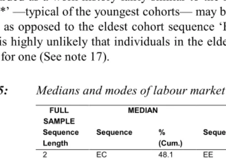
In any case, standard distribution-based methods will not work simply as a consequence of the complexity of the analysis. In our sample, the probability that each two sample members can be represented by different sequences of states will almost always be close to 1. Moreover, given that sequences do not have a numerical meaning, we can not use the mean of the distribution of sequences as the mid-point of the distribution. For this reason, Table 5 shows both the median sequence and the mode sequence of the distribution of the full sample as well as that of the five cohorts for different sequence lengths. This procedure has allowed us to detect relevant regularities which are presented below (See note 15). We first present results for the whole sample, and, then, compare typologies of sequences by cohorts.
For the full sample, the most frequent sequence up to seven spells corresponds to full stability in employment by job-to-job movements. The presence of this pattern quickly decreases with the sequence length (for instance, while among two-spell sequences the pattern “EE” accounts for 45.1% of the observations, among five-spell sequences the pattern “EEEEE” only accounts for 10.6%). As regards eight-spell sequences, the mode corresponds to exhibiting only two successive employment spells (with a frequency of 4.0%). We have checked that the pattern ‘EE·’ corresponds to sample members who have reached the moment of the survey in their second spell.
Results clearly differ by cohorts. In particular, they show that the patterns for the total sample are originated by the behaviour of the youngest cohorts. The youngest cohorts (third, fourth and fifth ones) show the two following main patterns: a history containing two spells (‘EE·’) and a history of successive jobs (‘EEEE*’), where ‘*’ means that successive spells have the same employment status as the last one. The former pattern constitutes a non-finished work-life experience since all of them fall below the mandatory retirement age (between 33 and 62 years-old).
sequences, 53.8 per cent of ‘EE’ sequences corresponds to males. Thus, the minor presence of the pattern ‘EB’ for the youngest cohorts might be due to the fact that women are showing work-life histories more similar to those of men.
As regards five and six-spell sequences, it is also possible to detect some life cycle patterns. On the one hand, there are two clear patterns in the first and second cohorts: a two-spell history (‘EA·’) and a four-spell history (‘E0EA·’). Both are non-complete work histories, but they are similar considering that the zero of the second history corresponds to National/War Service. Therefore, those two patterns are actually quite similar. If there was a recall bias affecting the answers of the eldest cohorts —which would then collapse successive employment spells into only one— the two eldest cohorts’ patterns ‘EA·’ and ‘E0EA·’ might be regarded as similar to the most frequent patterns of the youngest cohorts (‘EE·’ and ‘EEEE*’). As explained in Section 2.1 above, previous research about recall bias using the BHPS has not found in particular this kind of bias (see note 16). Nonetheless, it is likely that the eldest cohorts forget shorter employment spells more easily, remembering the longest employment spells with higher probability (as Booth et al., 1999 remark). In addition, since for the youngest cohorts these shorter employment spells must be closer in time than for the eldest ones, they would be more likely included in the pattern of successive employment spells. As a consequence, having only two employment spells (‘EE·’) can be regarded as a work-history fairly similar to the sequence ‘EA·’. However, the mode ‘EEEE*’ —typical of the youngest cohorts— may be suggesting a new work-life history pattern as opposed to the eldest cohort sequence ‘E0EA·’, the reason lying on the fact that it is highly unlikely that individuals in the eldest cohort have forgotten every spell except for one (See note 17).
Table 5: Medians and modes of labour market status sequences
FULL SAMPLE
MEDIAN MODE
Sequence Length
Sequence % (Cum.)
Sequence %
2 EC
ED
48.1 54.9
EE 45.1
3 EDD
EDE
49.1 54.9
EEE 25.0
4 EDEA 49.9 EEEE 15.6
5 EDEBB 50.0 EEEEE 10.6
6 EDEBBE 50.0 EEEEEE 7.4
7 EDEBBEB 50.0 EEEEEEE 5.3
8 EDEBBEBE 50.0 EE·
EEEEEEEE 4.0 3.4
1st. COHORT
2 EA
EB
39.9 62.9
EE EB
5 EBEED EBEEE 44.4 50.5 EEEEE E0EEE EBEEE EBEBE 7.7 6.2 6.1 4.8 6 EBEEED EBEEEE 46.8 50.5 EEEEEE E0EEEE EBEEEE [EA·] 5.6 4.9 3.6 [1.5] 7 EBEEEEA EBEEEEE 48.2 50.5 EEEEEEE E0EEEEE [EA·] 4.2 3.7 [1.5] 8 EBEEEEEA EBEEEEEE 49.0 50.5 EE· EEEEEEEE [EA·] 2.8 2.7 [1.5] 4th. COHORT 2 ED EE 44.1 100 EE EB 55.9 23.1 3 EDE EE· 44.1 51.2 EEE EBE [E0E] 33.5 20.0 [0.9] 4 EDEE EE· 44.1 50.7 EEEE EBEE 24.0 11.8 5 EDEEE EE· 44.1 50.7 EEEEE EBEEE EE· 16.7 7.0 6.6 6 EDEEEE EE· 44.1 50.7 EEEEEE EE· EBEEEE 12.0 6.6 4.2 7 EDEEEEE EE· 44.1 50.7 EEEEEEE EE· [EA·] 8.6 6.6 [0.2] 8 EDEEEEEE EE· 44.1 50.7 EE· EEEEEEEE 6.6 5.7 5th COHORT 2 ED EE 45.9 100 EE EB 54.1 17.3 3 EDE EE0 45.9 53.7 EEE EBE 33.8 13.4 4 EDEE EE· 45.9 53.3 EEEE EE· EBEE 22.3 7.5 7.1 5 EDEEE EE· 45.9 53.2 EEEEE EE· 15.9 7.4 6 EDEEEE EE· 45.9 53.2 EEEEEE EE· 11.6 7.4 7 EDEEEEE EE· 45.9 53.2 EEEEEEE EE· 8.4 7.4 8 EDEEEEEE EE· 45.9 53.2 EE· EEEEEEE E 7.4 5.0 Notes:
An additional remarkable aspect in Table 5 is the movement of the median closer to the mode for the youngest cohorts. A plausible interpretation for this result lies on the fact that the distribution of sequences has changed, so that histories are more linked to the labour market (See note 18) and, in addition, sequences which are more homogeneous than before are being observed (See note 19).
Table 6: Medians and modes of four-spell sequences by cohort and involuntary
job separations
Separation Status Full Sample 1st COHORT 2nd COHORT Median (%C) Mode (%) Median (%C) Mode (%) Median (%C) Mode (%)
Ever Involuntary Separated EDED (45.7) EDEE (51.0)
EEEE (21.9) EBEE (6.5)
EBEE (49.7) ECE0 (50.5)
EEEE (9.3) E0EE (6.3) EBEE (6.3) EBED (49.1) EBEE (53.9) E0EE (15.7) EEEE (13.9) Never Involuntarily Separated ECDC (49.7)
ECDE (50.1) EEEE (12.5) EBEE (9.0) EBB0 (48.8) EBBA (50.9) EBEB (6.8) EEBE (6.4) EBE0 (47.5) EBEA (51.7) EBEB (7.2) EBEE (6.7)
Separation Status 3rd COHORT 4th COHORT 5th COHORT Median (%C) Mode (%) Median (%C) Mode (%) Median (%C) Mode (%)
Ever Involuntary Separated EDED (49.6) EDEE (52.1) EEEE (16.3) E0EE (11.1) EEBD (43.7) EEBE (51.3) EEEE (32.3) EBEE (8.4) EDEE (49.5) EE00 (50.0) EEEE (26.9) EDEE (9.0) Never Involuntarily Separated EBED (41.9)
EBEE (54.6) EBEE (12.6) E0EE (9.7) EDEE (46.2) EE00 (56.0) EEEE (19.5) EBEE (13.6) EDEE (43.9) EE00 (55.2) EEEE (19.8) EE00 (11.3) Notes:
%C = Cumulative percentage. % = Frequency
Finally, we introduce a distinction between individuals who have ever been involuntarily separated and individuals who have not in Table 6. This Table shows the medians and modes for the full sample and for each of the five cohorts. Only four-spell sequences are displayed, since patterns were clear enough for sequences with more spells. Sequences in both groups are rather similar in the fourth and fifth cohorts. However, they clearly differ from those in the eldest ones. Among the latter, the mode of those who have never been involuntarily job exhibits the pattern ‘EB’ in the first two spells which, as was explained above, corresponds to a typical female pattern.
3. Estimation of the differences along the life cycle: Sequence
analysis
In this section we apply an optimal matching analysis (OMA) which draws from techniques used in DNA sequence matching (note 20). It was first introduced to the social sciences by Andrew Abbot (note 21), who has applied OMA to a range of sociological issues, such as the development of the welfare state and musicians’ careers (note 22). The technique has also recently been utilized to study social mobility (note 23) and to examine other social and political processes (note 24).
3.1. Alternative methods
Researchers with sequence data sets have at their disposal a variety of methods to be applied. Those methods can be classified in two types: step-by-step methods and whole sequence methods. Among the first group we encounter time series, Markovian and event history methods. Time series are applied when the interest is to find a simple stochastic generator that effectively fits entire sequences (which may involve auto-regression, moving averages or both; see note 25). Markov methods are applied in order to fit sequences of categories by estimating transition probabilities step by step (note 26). Finally, event history methods are used when the researcher’s interest focuses on transitions from only one particular prior category and when the issue is time until transition (note 27).
For those reasons, instead of taking our OMA results as input to some additional descriptive analysis (such as is usually done with clustering algorithms), we will show in section 3.5 below which individual and job-related characteristics lie behind the estimated measure of distance resulting from our OMA application.
3.2. Background: The basics of Optimal Matching Analysis (OMA)
Let us briefly make a comment on the intuitive idea underlying this process of optimal
matching (See note 28). We consider sequences of states which are elements of a finite
space state, say 7777. S denotes the set of all finite sequences over 7777, meaning that:
if aÎS then a=(a1,...,an) with a1,...,an Î7777
n= |a| is the length of the sequence. We desire to compare two sequences a,b ÎS. The basic idea is to define a set of elementary operations which can be used sequentially to transform one sequence until it becomes equal to the other sequence.
Let Z denote the set of basic operations and a(w) the sequence resulting from a by applying the operation w ÎZ. We consider three elementary operations:
a) Insertion: a(i) denotes the sequence resulting from a ÎS by inserting one new element (a state from 7777) into the sequence a.
b) Deletion: a(d) denotes the sequence resulting from a by deleting one element from this sequence.
c) Substitution: a(s) denotes the sequence resulting from a by changing one of its elements into another state.
We can think of sequentially applying elementary operations to a given sequence.
Let a(w1,w2,...,wk) denote the new sequence resulting from a by applying first the
elementary operation w1, then w2, and so on until finally wk. Then, given two sequences,
a,b ÎS, we can ask for a sequence of elementary operations which transform a into b. In general, there will be many such sequences of elementary operations which transform a into b. Now, the intuitive idea for developing a distance measure for sequences is to look for the shortest sequence of elementary operations which transform
[
]
[ ]
c w w
w
kc w
ii k
1 2
1
,
,...,
=
=
å
(1)Setting c[] = 0 for no operation, we can formally define:
( )
a
,
b
=
min
{
c
[
w
1,
w
2,...,
w
]
|
b
=
a
[
w
1,
w
2,...,
w
]
,
w
Î
Z
,
k
³
0
}
d
Z k k i (2)to measure the distance between the sequences a and b. This measure is by definition non–negative, and
d
Za
,
b
= 0 only if a = b (See note 29).“Optimal matching” without further qualification normally means referring to this
distance measure based on Z={i,d,s} resulting in a metric distance. Of course, the distance measure also depends on the definition of the cost functions c[w]. These cost functions can be arbitrarily defined (as we will see below) with respect to the intended applications. As a special case, one can set:
c(i)=c(d)=1, and c(s)=2 (3)
The distance between two sequences a and b is then simply the number of indel operations (insertions and deletions) which are necessary to transform one sequence into the other. Once the costs of those three basic operations are established, the algorithm evaluates all posible solutions for each pair of sequences and returns the cost of the most efficient transformation path as the “distance” between the sequences. Pairs of sequences with small “distances” are similar to one another, while pairs with larger “distances” are more distinct.
An example that will show how this optimal alignment method uses the set of operations to align and transform pairs of sequences is the following. Consider two hypothetical sequences in Table 7.
Table 7: OMA Example (I)
POSITION 1 2 3 4 5 6 7 8 9 10 11 12 13 14 15 16
In the comparison of Sequences 1 and 2, we find discrepancies in elements 1-5, 9-11, and 14. We could use a transformation that entails a series of substitutions. This would involve, for instance, substituting the 3 3 3 3 in elements 1-4 of the second sequence for the 4 4 4 4 in the first sequence, along with other substitutions later in the sequence. The cost of each individual transformation (e.g., substituting a 3 for 4 in the second element) is set by a-priori established costs of the different transformation operations. If we imagine that the cost of substituting one element for another is the difference in their numeric values (w(ai,aj)=| ai- aj|) then the minimum total cost of
aligning the sequences is simply the sum of the individual operations; here, the “distance” between the sequences would equal: (4*|3-4|)+(|3-5|)+(|5-6|)+(|1-6|)+(|6-1|)=17.
The algorithm could also conceivably try a transformation strategy that involves insertions, deletions and substitutions. In this comparison, we could delete the 1 in element 14 of Sequence 1, shift the remaining 13 elements one position to the right and then insert a 3 in the first element (Table 8).
Table 8: OMA Example (II)
POSITION 1 2 3 4 5 6 7 8 9 10 11 12 13 14 15 16
Sequence 1: 4 4 4 4 5 5 5 5 6 6 6 6 6 1 1 1 (original)
Sequence 1a: 3 4 4 4 4 5 5 5 5 6 6 6 6 6 1 1 (after insertion and deletion) Sequence 2: 3 3 3 3 3 5 5 5 5 1 6 6 6 6 1 1
3.3. Optimal matching parameters: Substitution costs
Insertion and deletion costs are always identical in the algorithm used in this paper — which is described in the Appendix— and called indel cost (See note 31). However, the setting of substitution costs between sequence elements —i.e., the different labour market states— involves, in general, serious consideration of theoretical questions. Optimal matching requires an explicit parameterization of substitutions, since substitution costs may affect distances. One can use a default cost function where indel cost equals 1 and substitution cost equals 2. In this case, the alignment of two sequences provides, then, the longest common subsequence (See note 32). This option is an interesting starting point because it makes a substitution equivalent to two indel operations —a deletion followed by an insertion; that is, both cost the same. However, we consider that, in our case, the initial basis for setting those costs should be related to the relative importance of changing the labour market states along the work history of the individual. Even though the data shows numerous moves across labour market states in the period of observation some labour market moves involve a substantial change in the degree of attachment to the labour market, when compared to other types of changes. That is, some pair of states seem to be fairly closely connected by career mobility than others. It seems necessary, therefore, to add mobility information to our measures of state resemblance or dissimilarity.
Doing that involved the use of two different “distance” matrices. For the first of those matrices, substitution costs is calculated as the absolute difference w(ai,aj)=| ai
-aj|; the underlying assumption for this is based on the fact that it is desirable that two
states are more similar the less drastic the associated change between the correspondent labour market states. That is, not all substitutions really “cost” the same. The difference between a state of “Out of labour force” (code A in Table 2) and a situation of “Employment” (code E) is greater than the difference between “Out of labour force” (code A) and a state of “Full time student” (code C). This fact explains why we should differentiate the costs of substitution. Work-life histories involving status changes characterized by low “vertical” distances across occupations will then be closely linked by the matching algorithms.
this particular weakness of the matching method is to use whatever empirical data the researcher has available. In our case, this involved producing a “distance” matrix based on mobility information by creating a matrix of transitions between the different values of the labour market statuses (as defined in Table 2). To explain this idea, let us assume a sample of i=1,...,n sequences: yi=(yi1, yi2,..., yiT), where the elements are valid statuses
in the state space 7777={ 1,...q }. We can then define:
Nt(x)= Number of sequences being in state x at t
(4)
Nt,t’(x,y)= Number of sequences being in state x at t and in state y at t’
(5)
Those quantities can be used to construct the referred substitution cost matrix; the underlying intuition is that two statuses are less different when there are, in the dataset, more transitions from one status into the other. One way of using this information about transitions would be to use:
p x y
N
x y
N x
t t t T t t T( , )
( , )
( )
,=
= + -=-å
å
1 1 1 1 1 (6)in order to define substitution costs as follows:
j i i j j i j
i
b
p
a
b
p
b
a
if
a
b
a
w
(
,
)
=
2
-
(
,
)
-
(
,
)
¹
(7)j i j
i
b
if
a
b
a
w
(
,
)
=
0
=
(8)3.4. Optimal matching analysis results
Given a model of substitution costs, we can apply the optimal matching algorithm to our data. Pair-wise comparison of n sequences requires n(n-1)/2 alignments. However, as Abbot and Forrest remark (1986), there is an inherent problem with analyses which involve procedures of pair-wise comparison: the processing time required rises with the square of, rather than in direct proportion to, the number of cases (see also Halpin and Chan, 1998). If n is big and if sequences are particularly long —as in our dataset— this results in strong constraints on the size of the sample we can deal with. We managed to circumvent this problem by taking into account the aim of our research: to analyse how much life cycle work-histories are disrupted by involuntary job separations. If we had calculated distances between all pair of sequences in our sample —apart from the computational burden involved— this would have offered no measure of dissimilarity between the two relevant sub-samples (ever involuntary job separated and the remainder of the sample). Thus, rather than calculating distances between all pairs of sequences, here we calculated the distance between each sub-sample’s sequence and each of the median sequences in each cohort. Given that the deviation of the distribution of sequences from the mean is likely to be of considerable magnitude (see previous Section 2.2), we regard the median sequence in each cohort as the centre of the distribution, thereby providing an idea of the typical work-history in the cohort. In addition, this procedure allowed us to substantially reduce the computational intensity of the task, and to deal with an eventual ‘right-censoring’ bias affecting the length of sequences (given that we compare sequences inside each cohort, the censoring problem is mitigated, as we explained in previous sections).
dissimilarity index, a means contrast is reported in the last column of the table, in order to statistically check the differences by those sub-samples (EINV0 and EINV1).
In general, Table 9 shows that involuntarily job separated men are clearly more different from their respective median life-cycle sequence, except for the youngest cohort. A similar result is obtained for women: ever-separated women are comparatively more different when compared to their median sequence than their non-separated counterparts.
Therefore, involuntary job separations give way to employment status sequences which clearly differ from the median employment status sequence in each cohort. In addition, the distance to this median sequence is comparatively larger for individuals who have ever involuntarily job separated. The only exception is that of men in the fifth cohort. Our interpretation of those results is as follows. Remember that although this fifth cohort was born in the fifties, the starting average year of their first spell was 1972 (see Table 1). Given that their life course started at the beginning of the oil crises, they were presumably affected by the employment flexibility policies characteristic of the eighties. However, women in the fifth cohort do not exhibit such a modification in estimated distances when compared to the behaviour of the previous cohorts. Thus, from a historical perspective, involuntary job separations have remarkably modified men’s life cycles: in particular, they have given way to sequences which are significantly different from the ‘typical’ life cycle of their respective cohort (i.e., the median sequence). However, for the youngest men (i.e., those who were born between 1950 and 1959) the fact of suffering an involuntary job separation at some point in time appears as more connected (or more similar) to the ‘typical’ life cycle.
3.5. OLS regressions on sequence dissimilarities
Table 9: Average optimal dissimilarity index to median sequences (by gender and cohort). Total Sample
Substitution cost matrix:
Average dissimilarity index T-test Average dissimilarity index T-test
Default Men Women
EINV0 EINV1 EINV0 EINV1
Cohort 1 3.19 4.57 -4.56*** 3.37 4.93 -5.76***
Cohort 2 3.42 6.15 -9.92*** 5.99 6.46 -2.15**
Cohort 3 4.41 5.76 -6.74*** 4.50 5.51 -3.99***
Cohort 4 2.94 6.23 -12.04*** 4.25 5.34 -4.85***
Cohort 5 5.91 5.37 3.11*** 4.78 6.74 -8.54*** Absolute value
Cohort 1 2.88 4.21 -4.61*** 3.08 4.62 -5.83***
Cohort 2 3.38 6.11 -10.07*** 5.56 5.91 -1.76*
Cohort 3 4.09 5.24 -5.86*** 4.37 5.37 -3.96***
Cohort 4 2.87 6.17 -12.01*** 4.10 5.13 -4.71***
Cohort 5 5.67 4.59 6.59*** 4.31 6.17 -8.41*** Data-based
Cohort 1 2.91 4.25 -4.53*** 2.95 4.39 -5.36***
Cohort 2 3.35 6.13 -10.19*** 5.10 5.02 0.55
Cohort 3 3.77 5.09 -6.87*** 3.83 4.88 -4.18***
Cohort 4 2.85 6.15 -11.97*** 3.56 4.63 -4.93***
Cohort 5 5.62 4.43 7.58*** 1.74 3.13 -6.98***
Notes:
The figures in this table indicate each cohort’s optimal distance by sex to the median sequence inside each cohort (for individuals either ever involuntarily separated or not).
Table 10: Average optimal dissimilarity index to the median sequences (by sex and cohort). Only individuals with completed life cycles
Substitution cost matrix: Average dissimilarity index T-test Average dissimilarity index T-test
Default Men Women
EINV0 EINV1 EINV0 EINV1
Cohort 1 6.96 4.18 8.89*** 3.64 5.05 -5.28***
Cohort 2 3.12 5.84 -9.95*** 5.25 5.56 -1.49
Cohort 3 3.81 5.90 -5.32*** 4.13 4.91 -2.77**
Cohort 4 4.87 5.07 -0.38 6.86 6.08 1.00
Cohort 5 8.61 7.25 1.48 8.17 4.80 3.38*** Absolute value
Cohort 1 6.79 4.18 8.40*** 3.64 4.64 -3.71***
Cohort 2 3.11 5.84 -10.00*** 4.81 5.05 -1.29
Cohort 3 3.51 5.61 -5.58*** 4.02 4.79 -2.78***
Cohort 4 4.49 4.61 -0.21 6.31 5.69 0.89
Cohort 5 7.78 6.24 2.18 7.57 4.64 3.45** Data-based
Cohort 1 6.12 4.18 6.25*** 3.61 4.04 -1.68*
Cohort 2 3.11 5.83 -9.99*** 4.61 4.50 0.67
Cohort 3 3.49 5.71 -5.79*** 3.59 4.19 -2.26**
Cohort 4 4.52 4.62 -0.19 6.23 5.24 1.36
Cohort 5 8.07 6.19 2.54* 7.98 4.43 3.55**
Notes:
The figures in this table indicate each cohort’s optimal distance by sex to the median sequence inside each cohort (for individuals either ever involuntarily separated or not).
Regarding gender, this dummy variable (itself or its interaction with involuntary job separations) does not significantly affect dissimilarity indices. Therefore, gender is not a key variable (in the present) to detect significant changes from the median employment status sequence in each cohort. We consider this to be a result arising from the increasing similarity of male and female histories detected in previous sections (See note 36).
Table 11: OLS Estimates for Dissimilarity Indices
SUBSTITUTION COST MATRIX
Absolute Value Default Data-Based
N=6159 N=6159 N=6159
Variable Coeff. T-ratio Coeff. T-ratio Coeff. T-ratio
Race (Whites=1) .02 0.08 .02 0.11 .07 0.35
Years since the first spell -.01 -1.44 -.01 -1.33 -.01 -2.59***
Cohorts: Cohort1 Cohort2 Cohort4 Cohort5 -.82 .66 -.40 .33 -3.72*** 3.36*** -2.29** 1.71* -.71 .84 -.46 .53 -3.10*** 4.10*** -2.52** 2.65*** -.55 .59 -.41 .38 -2.56 3.13*** -2.39** 2.04**
Involuntary job separation .82 4.77*** .81 4.59*** .78 4.70***
Gender (Males=1) .01 0.07 .06 0.35 -.01 -0.08
Education: Higher and first degree Teaching, nursing and other GCE A level or equivalent GCSE O level or equivalent Vocational training .17 .06 -.01 .02 -.10 1.26 0.68 -0.05 0.25 -0.82 .24 .05 -.02 .01 -.11 1.68* 0.53 -0.15 0.13 -0.88 .16 .04 -.08 .04 -.07 1.20 0.46** -0.56 0.44 -0.58
Mandatory retirement age .05 0.28 .02 0.14 .17 0.98
Interactions: Invol. Separated*Cohort1 Invol. Separated*Cohort2 Invol. Separated*Cohort4 Invol. Separated*Cohort5 .13 .30 .44 -.56 0.51 1.34 2.11** -2.70*** .19 .34 .43 -.38 0.69 1.47 1.99** -1.74* .09 .17 .44 -.74 0.34 0.77 2.14** -3.67*** Interactions:
Invol. Separated*Gender -.01 -0.07 .05 0.35 .09 0.67
Interactions: Gender*Cohort1 Gender*Cohort2 Gender*Cohort4 Gender*Cohort5 -.12 -.73 -.23 .16 -0.50 -3.31*** -1.05 0.75 -.23 -1.07 -.34 .02 -0.89 -4.71*** -1.52 0.10 -.03 -.46 -.06 .29 -0.13 -2.16** -0.30 1.41
Constant 4.59 14.22*** 4.79 14.39*** 4.37 13.96***
R2 0.06 0.07 0.06
F-value 18.47*** 20.78*** 16.85***
Notes: Reference individual is woman, not white, belongs to Cohort 3, has never been involuntarily-job separated, has CSE, Scot Grade or no qualification, and has not yet reached the mandatory retirement age (60 for women and 65 for men). * = Significant at 0.10 level
** = Significant at 0.05 level *** = Significant at 0.01 level or better
4. Conclusions
employment status mobility from a life-cycle perspective. Involuntary job separations, gender and birth cohort are the three variables on which our research focus has centered. We make two principal contributions. First, we have used an alternative methodological approach (optimal matching analysis) to demonstrate the existence of a systematic impact of involuntary job separations on life course mobility. This procedure allowed us to better understand the factors that influence the mobility across various stages of the life course for five different cohorts.
Our second contribution has been to provide new information about historical employment mobility changes in Britain, placing a special focus on the incidence and consequences of involuntary job separations. Several main findings are worth underlying from this empirical sequence analysis:
- Older cohorts have fewer spells and less changes of employment status between successive spells. On the contrary, younger cohorts have more spells, they are more mobile —although their greater mobility does not include job-to-job movements— and present more homogeneous histories. Therefore, mobility in employment status has increased along the twentieth century.
- The historical change in female participation in the labour market would help to explain this increase in mobility, given that women sequences have become more similar to those of men.
- Birth cohorts in the second half of the century have been comparatively more affected by involuntary job separations, when compared to the eldest cohorts.
- Applying OMA techniques we find that there is a significant difference in employment status sequences between those individuals who have ever been involuntarily job separated and those who have not. In particular, involuntary job separations give way to employment status sequences which substantially differ from the median sequence in each cohort, however this effect is not constant across cohorts (and it is very small for the fifth cohort).
- Differences in sequences obtained applying OMA show that male employment sequences are more affected by involuntary job separations in the youngest cohort. That is, experiencing involuntary job separations becomes more ‘natural’ for men along the seventies. However, the gender differences are not confirmed in the regression analysis, corroborating that (ceteris paribus) women sequences are equal to those of men.
century and is now more affected by involuntary job separations. Evidence on a historical change in labour market participation of women is shown through increasing similarity between men and women employment status sequences. Therefore, the approach followed in this article has provided relevant (and previously unknown) information about the historical changes of employment status mobility in Britain, in special underlying the increasing importance of involuntary job separations.
5. Acknowledgements
Notes
1. See Mincer and Polachek (1974 and 1978), Corcoran and Duncan (1979), Goldin (1989), or Hill and O’Neill (1992).
2. See, for instance, Jacobson et al. (1993) for the US and Elias (1997) for the UK. 3. See, for instance, Hildreth et. al (1998) or Booth et. al (1999), who also use data
from the British Household Panel Survey.
4. See, in this respect, Abbot (1985), and Abbot and Forrest (1986).
5. Individuals under 34 years-old at 1-December-93 were also initially included in the analysis. Nonetheless, due to the short length of their observed work-histories, no significant results were attained regarding this sixth cohort. Therefore, they were excluded from the empirical analysis.
6. See Halpin (1997a) and Taylor (1996) for more complete details about the BHPS. 7. Following Halpin (1997a) suggestions, we have used the weights supplied in the
main database. As the job history information is included in our data files, the weight variable used has been CXEWGHT which selects the survey respondents and allows to adjust the sample selection and attrition effects. We have preferred the selection of survey respondents, because the proxies could not give accurate information on employment and job histories. On the weights variables in the BHPS and how to use them, see Taylor (1997).
8. See Elias (1991) and Elias (1997a).
9. As we will see, our findings on employment status mobility patterns can also be interpreted in the light of the historical process of the increasing participation of females in the labour market, in addition to those exogenous macroeconomic phenomena. This fact stresses, again, the importance of analyzing the evolution along time of the different birth cohorts.
10. The usual mobility measures in the literature are net mobility indicators. That is, they compare employment status in two different states (Elias, 1997b). On the other hand, the two measures we propose for mobility allow to attain a vision of the life cycle in the long-term.
Secondly, the remainder of reasons (presumably voluntary): promoted/left for a better job; took retirement; left to have a baby; and children/home care.
12. As it is well-known, very complex element schemes may retain important substantive information, but they also increase the computational intensity of the analyses, and may make it difficult to identify similar sequential patterns; conversely, overly simple schemes may disguise meaningful variation in sequential pattern.
13. Its rank is between 0 and 38 and it must be always lower than the number of spells of the individual.
14. Moreover, the gross mobility measure seems to decrease for the youngest cohorts. However, the shortest time period considered for those cohorts might be explaining this relationship.
15. This is a straightforward tool for studying labour market attachment: since we dispose of a set of discrete events, we can write down all of their logical combinations and then count the frequency of their occurrence in each sample (Berger, Steinmuller and Ziegler, 1993, and Hogan, 1978).
16. Instead, previous research has detected an under-reporting of unemployment spells, especially the shortest ones —see, for instance, Dex and McCulloch, 1997, and Elias, 1997a.
17. Given that this highly unlikely event would constitute the main argument in order to be able to assimilate this second group to the pattern of the eldest cohorts described above, this exploratory analysis allows us to state that this second group might be showing a new pattern of employment status mobility.
18. At least in their first spell, since the order of sequences to obtain medians is lexicographic.
19. The most frequent sequences up to four spells represent almost 50 per cent for the fifth cohort, while for the eldest cohorts they only represent less than 25 per cent. 20. See Sankoff and Kruskal, 1983.
21. Abbot and Forrest, 1986.
24. Baizán, Michielin and Billari, 2002; Solís and Billari, 2002. See also Billari (2001) and Billari and Piccareta (2001) for respective discussions of the sequence analysis approach to the study of life courses.
25. See Isaac et al. (1991) and Box et al. (1994) in this respect. 26. Useful reviews are found in Bondon (1973) and Sterman (1976). 27. A review of this method is found in Yamaguchi, 1991.
28. Appendix B gives a full account of the mathematical algorithm used by optimal matching.
29. Symmetry does not automatically hold, but can be forced by equating insertion and deletion costs, or by a slightly different definition: minimum cost of transforming a
into b or b into a. Whether the distance measure will also be transitive, and thus constitutes a metric distance, depends on the definition of the set of elementary operations, Z. Transitivity is automatically guaranteed for the simple case when there are only insertions, deletions and subtitutions.
30. In many applications, the cost of insertions and deletions are fixed at a value slightly higher than the highest substitution cost (see Abbott and Hrycak, 1990). 31. Insertion and deletion costs may themselves vary. However, these costs are in some
sense a function of what the sequence already looks like; because of this uncertainty, most applications make indel costs the same in all cases (see Abott and Hrycak, 1990, pp. 155).
32. The relationship is as follows: length of longest common subsequence=0.5*
(m+n-d(a,b)), where d(a,b) is the optimal matching distance when using the cost
functions as indicated in the text; m and n denote the length of the first and second sequence, respectively.
33. Results for the fourth and fifth cohorts must be cautiously analysed because their completed life cycles must be rather different from the completed life cycles of the remainder cohorts. Due to their limited sample size, only occasionally the average dissimilarity measures are significantly different for individuals ever and never involuntarily job separated in those two youngest cohorts.
34. McVicar et. al (2001, pp. 325) also make use of regression techniques with the output of optimal matching analysis, and indicate other papers adopting a similar approach.
a portion “unexplained” following the decomposition by Blinder (1973) and Oaxaca (1973). This allows us to test whether or not the effect of the remainder explanatory variables on the dissimilarity indices differs between those never involuntarily job separated and those ever involuntarily job separated. We have estimated separately OLS estimations for both groups, and have worked out the Oaxaca-Blinder decomposition. In addition, given that individuals might not be randomly distributed to those groups, we have tested whether or not there is selection by workers into both subgroups. A two-stage Heckman procedure was applied for this purpose. The most relevant result is that having been involuntarily job separated is by far the chief factor explaining individuals’ distance to the median sequences in each cohort. Those results are not shown, but are available from the authors upon request. Moreover, it is observed that distances to the median sequence are almost unrelated to the explanatory variables. This fact may explain the low R2 values showed in Table 11. That is, the variables introduced in the model —in order to control for initial conditions and for other aspects which remain constant along time— explain less than 10 percent of the individuals’ work-history. The remainder 90 percent is then explained by other factors, such as luck, the historical moment, and the decisions that each individual takes along his/her life-course.
References
Abbot, A. (1985). “Sequence Analysis: New Methods for Old Ideas”, Annual Review of
Sociology, 21: 93-113.
Abbot, A. and J. Forrest (1986). “Optimal Matching Methods for Historical Sequences”, Journal of Interdisciplinary History, 16: 471-494.
Abbot, A. and Hrycak, A. (1990). “Measuring Resemblance in Sequence Data: An Optimal Matching Analysis of Musicians’ Careers”. American Journal of
Sociology, 96(1): 144–185.
Baizán, P., F. Michielin, and F.C. Billari (2002). “Political Economy and Life Course Patterns: The Heterogeneity of Occupational, Family and Household Trajectories of Young Spaniards”, Demographic Research, vol. 6, art. 8, 192-240.
Berger, P.A.,Steinmuller, P. and Ziegler, Z. (1993) “Upward Mobility in Organisations: The Effects of Hierarchy and Opportunity Structure”. European Sociological
Review, 9:173–188.
Billari, F.C. and R. Piccarreta (2001), "Life courses as sequences: an experiment in classification via monothetic divisive algorithms", in S. Borra, R. Rocchi,M. Vichi, M. Schader (Eds.), Advances in Classification and Data Analysis, Springer Verlag, Berlin and New York: 351-358.
Bondon, R. (1973). Mathematical Structures of Social Mobility, San Francisco: Jossey Bass.
Booth, A.L., M. Francesconi, and C. García-Serrano (1999). “Job Tenure and Job Mobility in Britain”, Industrial and Labor Relations Review, vol. 53, no. 1, 43-70.
Box, G.E.D, Jenkins, G.M. and G.C. Reisel (1994). Time Series Analysis, Englewood Cliffs, NJ: Prentice Hall.
Chan, T.W. (1994). Tracing Typical Mobility Paths. Ms. Nuffield Coll. Oxford.
Chan, T.W. (1995). “Optimal Matching Analysis: A Methodological Note on Studying Career Mobility”, Work and Occupations, 22 (4), 467-490.
Corcoran, M. and Duncan, G. (1979): “Work History, Labor Force Attachment, and Earnings Differences Between the Races and the Sexes”, Journal of Human
Creedy, J. and Disney, R. (1981): “Changes in Labour Market States in Great Britain”,
Scottish Journal of Political Economy, vol. 28, no. 1, February, pp. 76-85.
Dex, S. and McCulloch, A. (1997): “The Reliability of Retrospective Unemployment History Data”, Working papers of the ESRC Research Centre on Micro-Social
Change, paper 97-17 Colchester, University of Essex.
Elias, P. (1991). “Methodological, Statistical and Practical Issues Arising from the Collection and Analysis of Work History Information by Survey Techniques”,
Bulletin de Methodologie Sociologique, no. 31, 3-31.
Elias, P. (1997a): “Who forgot they were unemployed?”, Working papers of the ESRC
Research Centre on Micro-Social Change, paper 97-19 Colchester, University of
Essex.
Elias, P. (1997b): “Restructuring, Reskilling and Redundancy: A Study of the Dynamics of the UK Labour Market, 1990-95”, Working papers of the ESRC Research
Centre on Micro-Social Change, paper 97-20 Colchester, University of Essex.
Farber, H.S. (1994), "The Analysis of Interfirm Worker Mobility", Journal of Labor
Economics, 12, 554-594.
Goldin, C. (1989): “Life-Cycle Labor Force Participation of Married Women: Historical Evidence and Implications”, Journal of Labor Economics, vol. 7, no. 1, pp. 20-47.
Halpin, B. (1997a): “Unified BHPS Work-life Histories: Combining Multiple Sources into a User-friendly Format”. Technical Papers of the ESRC Research Centre of
Micro-Social Change. Technical Paper 13. Colchester, University of Essex.
Halpin, B. (1997b): “Is Class Changing? Evidence from BHPS Retrospective Work-life Histories”, Working papers of the ESRC Research Centre on Micro-Social
Change, paper 97-13 Colchester, University of Essex.
Halpin, B. and T. W. Chan (1998) Class Careers as Sequences: an Optimal Matching Analysis of Work-Life Histories , European Sociological Review, 14: 113-130. Hill, M.A. and O’Neill, J.E. (1992): “Intercohort Change in Women’s Labor Market
Status”, Research in Labor Economics, vol. 13, pp. 215-286.
Hildreth, A. K., S.P. Millard, D.T. Mortensen and M. Taylor (1998). “Wages, Work and Unemployment”, Applied Economics, vol. 30, 1531-1547.
Hogan, D.P. (1978): “The Variable Order of Events in the Life Course”, American
Isaac, L., S.M. Carlson and M.P. Mathis (1991). Quality of quantity in comparative
historical time series analysis, Presented at Soc. Sci. Hist. Assoc., New Orleans,
2, November.
Jacobson, L.S., R.J. Lalonde and D.G. Sullivan (1993): “Earning losses of displaced workers”, American Economic Review, 83, 4, pp. 685-709.
McVivar, D., and M. Anyadike-Danes (2002): “Predicting successful and unsuccessful transitions from school to work by using sequence methods”, Journal of the
Royal Statistical Association, Series A, 165, Part 2, pp. 317-334.
Mincer, J. and S. Polachek (1974): “Family Investments in Human Capital”, Journal of
Political Economy, 82 (March/April), pp. S76-S108.
Mincer, J. and S. Polachek (1978): “Women’s Earnings Reexamined”, Journal of
Human Resources, 13 (winter), pp. 118-133.
Sankoff, D. and J.B. Kruskal (1983). Time Warps, String Edits and Macromolecules, Reading, MA: Addison-Wesley.
Solís, F. and F.C. Billari (2002). “Work Lives amid Social Change and Continuity: Occupational Trajectories in Monterrey, México”, Max Planck Institute for Demographic Research, working paper WP 2002-009.
Stewman, S. (1976). “Markov Models of Occupational Mobility”, J. Math. Soc., 4: 201-45, 247-78.
Stovel, K., M. Savage and P. Bearman (1996). “Adscriptio into Achievement: Models of Career Systems at Lloyds Bank, 1890-1970”, American Journal of Sociology, 102: 358-399.
Taylor, M.F. (1997): “British Household Panel Survey User Manual”, User documentation, ESRC Research Centre on Micro-Social Change.