R E S E A R C H
Open Access
A priori
error analysis of stabilized mixed
finite element method for reaction-diffusion
optimal control problems
Hongfei Fu
1*, Hui Guo
1, Jian Hou
2and Junlong Zhao
1*Correspondence:
[email protected] 1College of Science, China
University of Petroleum, Qingdao, 266580, China
Full list of author information is available at the end of the article
Abstract
In this paper, we propose a novel stabilized mixed finite element method for the approximation of optimal control problems governed by reaction-diffusion equations. Compared with the classical mixed finite element methods, the main contributions of this paper are as follows. First, the novel method uses only one stabilization parameter which is not mesh-dependent, and, the new mixed bilinear formulation is coercive and continuous. Second, the novel method is easy to be implemented on a computer using the standard Lagrange finite element. Third, the solutions of the novel method to the optimal control problems require low
regularities. Fourth, the Ladyzhenkaya-Babuska-Brezzi (LBB) or the inf-sup condition for the mixed element spaces is unnecessary. Based on the novel method, we derive both continuous and discrete optimality systems for the corresponding constrained optimal control problems, and thena priorierror analysis in a weighted norm is discussed. Finally, numerical experiments are given to confirm the efficiency and reliability of the novel stabilized method.
Keywords: optimal control; reaction-diffusion equation; stabilized mixed finite
element;a priorierror analysis; numerical experiments
1 Introduction
Optimal control problems and their finite element solutions are attracting increasingly at-tentions of scientists and engineers. For systematic introductions of finite element meth-ods and their applications in solving optimal control problems, we refer the reader to [–].
In this paper, we are interested in the following distributed type optimal control prob-lem:
min u∈Uad
(y–yd)+
(σ–σd)+ γ
u, (.)
subject to a first-order mixed type reaction-diffusion equation
divσ+cy=f +Bu, in,
σ+A∇y= , in, (.)
and combined with homogeneous Dirichlet boundary condition
y= , on∂. (.)
Hereγ > is a penalty parameter, it is used to measure the relative importance of the terms appearing in the definition of the cost functional;Bis a linear operator;Uadis an admissible convex control set. Detailed information as regards this problem in a functional analysis setting will be discussed later.
This model problem plays an important role in many scientific and engineering appli-cations. For example, it can represent an optimal control of Darcy flows, where the pri-mal state variableymeans the pressure, the flux state variableσ stands for the velocity field, and the control variableuis an external force.A priorierror estimates of finite ele-ment approximations for optimal control problems governed by linear elliptic equations were studied extensively; see, for example, Refs. [, –]. Recently, mixed finite element method has also been found very useful in solving such optimal control problems which contain the flux state variable, see Refs. [–]. But all these works need a matched mixed finite element spaces for the state variable and its flux,i.e., LBB stability condition must be strictly satisfied. One of their best choices is the Raviart-Thomas (RT) element, see [], and therefore, the widely used Lagrange elements are excluded.
Inspired by the idea of so-called Galerkin least squares method, proposed by Hughes
et al. [] and theoretically analyzed by Franca and Stenberg [], and also the idea of so-called unusual stabilized finite element method [, ] for advection-diffusion equa-tions, we propose here a first-order mixed type stabilized finite element method for the elliptic optimal control problems. The novel method is proved to be efficient and reliable both in theoretical error analysis and numerical tests. It also embodies some advantages compared with the former work []: It uses only one stabilization parameter which is not mesh-dependent, however, the corresponding mixed bilinear formulation is still co-ercive and continuous; it is easier to be implemented using the standard Lagrange finite elements; it has relatively lower regularity requirements of the solutions to optimal con-trol problems; and it can be extended to solve optimal concon-trol problems governed by other type partial differential equations. Furthermore, compared with the classical mixed finite element method, it also has a free choice of mixed element spaces without the require-ment of LBB stability condition, and less degree of freedoms (DoFs) are adopted. Thus, it is more competitive in the practical computation and especially in the high-dimensional case.
2 Optimal control problems and optimality system
Letbe a bounded domain inRd(d≤) with Lipschitz boundary∂. LetThbe a fam-ily of regular triangulation of, such that=T∈ThT. DenotehTthe diameter of the elementT inTh, and seth=max
T∈ThhT. In this paper, we shall employ the usual no-tion for Lebesgue and Sobolev spaces; see Ref. [] for details. Throughout, letCdenote a strictly positive generic constant, not necessarily the same at each occurrence, but always independent of the mesh sizeh.
To give a detailed description of the model optimal control problem, let us define the state spaces
Y=H(), =L()d. (.)
and the control space
U=L(). (.)
Furthermore, letUadbe a closed convex subset of the control spaceU. In the following context, we will discuss some different cases on the choice ofUad.
In the following, we are ready to propose a simple but stable mixed numerical method. To this aim, we assumeA= (ai,j(x))d×dis symmetric and positive definite, and there exist positive constantsαandβsuch that
α|X|≤XTAX≤β|X|, ∀X∈Rd.
Besides, supposec=c(x) is bounded below and up by two constantsc∗andc∗such that ≤c∗≤c≤c∗.
We now first revisit the classical mixed formulation of problem (.)-(.): Find (y,σ)∈
L()×H(div;) such that for any (v,τ)∈L()×H(div;)
A–σ,τ– (y,divτ) + (divσ,v) + (cy,v) = (f+Bu,v). (.)
Then followed by integration by parts, and inspired by the stabilized finite element method [–], we propose a novel stabilized mixed weak formulation for (.)-(.): find (y,σ)∈Y×such that
Aδ(y,σ;v,τ) = (f+Bu,v), ∀(v,τ)∈Y×, (.)
where the mixed bilinear formulation
Aδ(y,σ;v,τ) =
A–σ,τ+ (∇y,τ) – (σ,∇v) + (cy,v)
–
T∈Th
δT
A–σ+∇y,τ–A∇v
T. (.)
Define the corresponding stabilization norm
{y,σ} δ=A–σ,σ+ T∈Th
δT(A∇y,∇y)T+ (cy,y). (.)
Then, we can easily derive the following coercive and bounded results.
Proposition .(Coercivity and boundedness) For <δ≤δT≤δ< ,we have Aδ(y,σ;y,σ)≥cδ {y,σ}
δ, ∀(y,σ)∈Y×. (.)
Moreover,for all(y,σ;v,τ)∈(Y×)
Aδ(y,σ;v,τ)≤Cδ {y,σ} δ {v,τ} δ. (.)
Hereδi(i= , )are two positive constants,cδ= –δand Cδ=max{, + /δ}.
Proof On the one hand, it follows from the definition that
Aδ(y,σ;y,σ)
=A–σ,σ+ (cy,y) – T∈Th
δT
A–σ,σ
T+
T∈Th
δT(A∇y,∇y)T. (.)
Hence, forδT≤δ< , the bilinear forma(,;,) is coercive onY×, and it satisfies
(.).
On the other hand, we conclude from (.) that
Aδ(y,σ;v,τ) =
A–σ,τ+ (∇y,τ) – (σ,∇v) + (cy,v)
–
T∈Th
δT
A–σ,τ
T+
T∈Th
δT(σ,∇v)T
–
T∈Th
δT(∇y,τ)T+
T∈Th
δT(A∇y,∇v)T. (.)
Note that
i
|aibi| ≤
i
ai
i
bi
.
Then for <δ≤δT≤δ< , we have
Aδ(y,σ;v,τ)
≤
A–σ,σ+ (A∇y,∇y) + T∈Th
δT(A∇y,∇y)T+ (cy,y)
×
A–τ,τ+ (A∇v,∇v) + T∈Th
δT(A∇v,∇v)T+ (cv,v)
≤
A–σ,σ+
+ δ
T∈Th
δT(A∇y,∇y)T+ (cy,y)
×
A–τ,τ+
+ δ
T∈Th
δT(A∇v,∇v)T+ (cv,v)
≤Cδ {y,σ} δ {v,τ} δ, (.)
which proves the boundedness result (.).
Proposition .(Existence and uniqueness) Assume the condition in Proposition.is valid.Furthermore,let f ∈L().Then for given control u∈L(),problem(.)admits a
unique solution(y,σ)∈Y×.
Proof Proposition . implies that the mixed bilinear formAδ(,;,) is coercive and
bounded in a weighted norm (.). Then the Lax-Milgram lemma implies the existence and uniqueness of the solution pair (y,σ)∈Y×. Furthermore, supposeu= in problem (.), we then have the following stability result with respect to the right-hand termf.
Proposition .(Stability) Let f ∈L().If the condition in Proposition.is valid,then
we have
{y,σ} δ≤C f L(), (.)
where the constant C depends on the Poincaré constant C,and the reciprocal of cδandδ.
Proof Let (v,τ) = (y,σ) in problem (.). Then it follows from Proposition ., the Poincaré inequality in Lemma ., and the definition of the stabilization norm that
cδ {y,σ}
δ≤ f L() y L()
≤C f L() ∇y L()
≤ C
√
δ
f L()
T∈Th
δT(∇y,∇y)T /
,
which implies the conclusion.
Denote
J(y,σ,u) =
(y–yd)+
(σ–σd)+ γ
u,
wherey=y(u) andσ=σ(u) areu-dependent.
Then for the given control setUad, we reformulate the optimal control problem (.)-(.) as follows: (OCP)
Jy∗,σ∗,u∗= min u∈Uad
such that (y,σ,u)∈Y××Uand
Aδ(y,σ;v,τ) = (f+Bu,v), ∀(v,τ)∈Y×.
It then follows from Ref. [] that the optimal control problem (OCP) has a unique solu-tion (y∗,σ∗,u∗)∈Y××Uad, and (y∗,σ∗,u∗) is the solution of (OCP) if and only if there is a pair of adjoint state (z∗,ω∗)∈Y×, such that (y∗,σ∗,z∗,ω∗,u∗)∈(Y ×)×U
ad satisfies the following optimality system: (OS)
State equation:
Aδ
y∗,σ∗;v,τ=f +Bu∗,v, ∀(v,τ)∈Y×. (.)
Adjoint state equation:
Aδ
v,τ;z∗,ω∗= –y∗–yd,v
–σ∗–σd,τ
, ∀(v,τ)∈Y×. (.)
Optimality condition:
γu∗–B∗z∗,u–u∗≥, ∀u∈Uad. (.) HereB∗is the adjoint operator ofB, which satisfies
(Bv,w) =v,B∗w, ∀(v,w)∈L()×H().
Remark . For the stabilization parameterδTbeing chosen as a constantδin the whole domain, the adjoint statesz∗andω∗in (.) satisfy the following strong forms:
–z= –(y–yd) –div(σ–σd), in,
z= , on∂, (.)
and
ω=∇z–σ–σd
–δ , in. (.)
In the following, we introducezandωbe the solutions of the dual problem such that
Aδ(v,τ;z,ω) = –(g,v) – (q,τ), ∀(v,τ)∈Y×. (.)
Then, similar to the proof in Proposition ., we have the following stability result.
Proposition .(Stability) Let g∈L()and q∈L()din problem(.).Assume the
condition in Proposition.is valid.Then we have
{z,ω} δ≤C g L()+ q L()d
, (.)
Remark . Letf,u∗ ∈L(). If the condition in Proposition . is valid, then from
Proposition . we have
y∗,σ∗ δ≤C f L()+u∗
L()
. (.)
Furthermore, letyd∈L() andσd∈L()d. Then from Proposition . and the above conclusion we have
z∗,ω∗ δ≤Cy∗–ydL()+σ∗–σdL()d
≤C f L()+u∗
L()+ yd L()+ σd L()d
. (.)
In the end of this section, we pay special attention on the solution of the variational inequality (.). It depends heavily on the structure of the convex setUad. For some cases (see,e.g.[, ]), we have the following explicit results.
CaseI.Uad=U Then the solution is
u∗(x) = γB
∗z∗(x). (.)
CaseII.Uad={u∈U:u≥, a.e. in} Then the solution is
u∗(x) =max
, γB
∗z∗(x). (.)
CaseIII.Uad={u∈U:a≤u≤b, a.e. in}where the boundsa,b∈Rfulfilla<b. Then the solution is
u∗(x) =max
a,min
b, γB
∗z∗(x). (.)
CaseIV.Uad={u∈U:
u≥}
Then the solution is
u∗(x) =max
, – γB
∗z∗(x)
+ γB
∗z∗(x), (.)
whereB∗z∗(x) =
B∗z∗(x) .
3 Stabilized mixed finite element approximation
In this section, we shall consider the approximation of problem (OCP) based on the novel stabilized mixed finite element method. As the bilinear formAδ(,;,) is coercive, there
In this work, we consider the approximations of the state and flux state variables in the following finite element spaces:
Yh=vh∈C() :vh|T∈P(T),∀T∈Th,vh= on∂
⊂Y, h=τh∈L() : (τh)i|T∈P(T),i= , , . . . ,d,∀T∈Th
⊂.
(.)
HerePkdenotes polynomials of total degree at mostk.
Furthermore, we consider piecewise constant elements for the approximation of the control variable, that is,
Uh=uh∈U:uh|T∈P(T),∀T∈Th
. (.)
LetUadh =Uh∩U
ad be the discrete admissible control set. It is apparently so thatUadh ⊂
Uad.
For the finite element spaces defined above, the stabilized mixed finite element approx-imation of (OCP), which will be labeled as (OCP)h, can be described as follows:
Jy∗h,σh∗,u∗h= min uh∈Uhad
J(yh,σh,uh), (.)
where (yh,σh,uh)∈Yh×h×Uhsatisfies
Aδ(yh,σh;vh,τh) = (f +Buh,vh), ∀(vh,τh)∈Yh×h. (.)
It is again well known (see Ref. []) that the optimal control problem (OCP)hhas a unique solution (y∗h,σh∗,uh∗)∈Yh×h×Uh
ad, and that a triplet (y∗h,σh∗,u∗h) is the solution of (OCP)h if and only if there is a pair of adjoint states (z∗h,ωh∗)∈Yh×h, such that (y∗
h,σh∗,zh∗,ω∗h,u∗h)∈ (Yh×h)×Uh
adsatisfies the following discrete optimality system: (OS)h
State equation:
Aδ
y∗h,σh∗;vh,τh
=f +Bu∗h,vh
, ∀(vh,τh)∈Yh×h. (.)
Adjoint state equation:
Aδ
vh,τh;z∗h,ω∗h
= –y∗h–yd,vh
–σh∗–σd,τh
, ∀(vh,τh)∈Yh×h. (.)
Optimality condition:
γu∗h–B∗zh∗,uh–u∗h
≥, ∀uh∈Uadh . (.)
Remark . The coercivity of the mixed bilinear formulationAδ(,;,) leads to a
posi-tive definite linear algebraic equation in the discrete level, and therefore, the discrete state and adjoint state equations (.)-(.) can be solved quickly using the popular solvers, such as the conjugate gradient (CG) solver and algebraic multi-grid (AMG) solver.
LetPhbe anL-projection fromU=L() toUhsuch that for anyu∈U
It is a matter of calculation that for the optimal controlu∗ ∈Uad, the projectionPhu∗ belongs toUh
ad. For example, we can give a proof for Case IV. In fact, letφ≡∈Uh in equation (.), then we have
Phu∗=
u∗≥, (.)
which proves the conclusion. The proofs of the other cases are similar. Besides, it is easy to check that
Phu|T=
|T|
T
u, ∀T∈Th, (.)
where|T|is the area of elementT.
Finally, similar to the explicit solutions (.)-(.) to the variational inequality (.) for different cases. The solution of (.) can also be described explicitly for the corre-sponding cases; see [, ]. We summarize them as below.
CaseI.Uadh =Uh Then the solution is
u∗h= γPh
B∗z∗ h
. (.)
CaseII.Uh
ad={uh∈Uh:uh|T≥,∀T∈Th} Then the solution is
u∗h=max
, γPh
B∗z∗ h
. (.)
CaseIII.Uad={uh∈Uh:a≤uh≤b, a.e. in} Then the solution is
u∗h=max
a,min
b, γPh
B∗z∗ h
. (.)
CaseIV.Uad={uh∈Uh:
uh≥}
Then the solution is
u∗h=max
, – γB
∗z∗ h
+ γPh
B∗z∗ h
. (.)
4 A priori error estimates
In this section, we shall givea priorierror estimates for the proposed novel stabilized mixed finite element method of optimal control problem.
Before that let us first recall the following interpolation and projection results.
Lemma .[] LetPhbe the L-projection defined in(.).Then for u∈H(),we have
Lemma . LetIh be the standard Lagrange interpolation operator defined in Ref. [].
Then there is a constant C> such that
v–Ihv L(T)+hT|v–Ihv|H(T)≤ChT|v|H(T), (.)
for∀v∈H(T),∀T∈Th.
Lemma .(Poincaré inequality) There is a positive constant Cwhich depends only on
the domainsuch that
v L()≤C ∇v L()d, ∀v∈H(). (.) In this paper, we aim to demonstrate the following main conclusion between the optimal solutions of (OS) and the stabilized mixed finite element solutions of (OS)h.
Theorem . Suppose that (y∗,σ∗,z∗,ω∗,u∗)and(y∗h,σh∗,z∗h,ωh∗,u∗h)are the solutions of
(OS)and(OS)h,respectively.Assume that the solutions{y∗,z∗} ∈H()∩H(),{σ∗,ω∗} ∈
H()d,and u∗∈H().Then there is a positive constant C such that
u∗–u∗
hL()+ y∗–y∗h,σ∗–σh∗ δ+ z∗–zh∗,ω∗–ωh∗ δ
≤Chu∗H()+
v=y,z;τ=σ,ω
v∗
H()+τ∗H()d
. (.)
Remark . Compared with Ref. [], a same optimal-order convergence between the exact solutions and numerical solutions is obtained. However, the requirement of reg-ularities for the flux stateσ∗ and adjoint flux stateω∗are both reduced fromH()dto
H()d. This appears to be a more realistic assumption if the original state equation is only
H-regular, and if the given dataf,yd,σdand the optimal controlu∗all belong toL(). In particular, for Cases I and IV, we can predict that the optimal controlu∗∈C∞() as if the given data are sufficiently smooth. Indeed, from (.) and (.) we can observe that the regularity of the optimal controlu∗agrees with that of the adjoint statez∗.
To derive the above main result, we introduce (yh(u∗),σh(u∗),zh(u∗),ωh(u∗))∈(Yh× h)as the discrete intermediate variables. They are associated with the optimal control solutionu∗∈Uadand satisfy
Aδ
yh
u∗,σh
u∗;vh,τh
=f+Bu∗,vh
, (.)
Aδ
vh,τh;zh
u∗,ωh
u∗= –yh
u∗–yd,vh
–σh
u∗–σd,τh
, (.)
for any (vh,τh)∈Yh×h.
For simplicity of presentation, below let us denote those solutions of (.)-(.) corre-sponding to the optimal controlu∗
(yh,σh,zh,ωh)
yh
u∗,σh
u∗,zh
u∗,ωh
u∗.
Lemma . Let(y∗h,σh∗,ωh∗,zh∗)and(yh,σh,zh,ωh)be the solutions of(.)-(.)and(.) -(.),respectively.Then the following estimates hold:
y∗h–yh,σh∗–σh δ+ z∗h–zh,ω∗h–ωh δ≤Cu∗–u∗hL(). (.)
Proof On the one hand, we conclude from (.) and (.) that
Aδ
y∗h–yh,σh∗–σh;vh,τh
=Bu∗h–u∗,vh
, ∀(vh,τh)∈Yh×h. (.)
Selectingvh=y∗h–yhandτh=σh–σhin (.). It then follows from the stability result in Proposition . that
y∗h–yh,σh∗–σh δ≤Cu
∗–u∗
hL(). (.)
On the other hand, we deduce from (.) and (.) that
Aδ
vh,τh;z∗h–zh,ω∗h–ωh
= –y∗h–yh,vh
–σh∗–σh,τh
, (.)
for any (vh,τh)∈Yh×h.
Letvh=z∗h–zhandτh=ωh∗–ωh. Following the stability result in Proposition . and the conclusion (.), we derive
z∗h–zh,ω∗h–ωh δ≤C y∗h–yh,σh∗–σh δ≤Cu∗–u∗hL(). (.)
Therefore, the proof of Lemma . is ended.
Then we turn to the validation of an optimal-order convergence between the interme-diate variables and the exact solutions.
Lemma . Let (y∗,σ∗,z∗,ω∗) and (yh,σh,zh,ωh) be the solutions of (.)-(.) and (.)-(.),respectively.Furthermore,assume the solutions{y∗,z∗} ∈H()∩H()and
{σ∗,ω∗} ∈H()d.Then the following estimates hold: y∗–yh,σ∗–σh δ≤Chy∗H()+σ∗H()d
, (.)
z∗–zh,ω∗–ωh δ≤Ch
v=y,z;τ=σ,ω
v∗H()+τ∗H()d
. (.)
Proof First of all, it is clear that (.) is the mixed finite element approximation of (.). Therefore, the result (.) can easily be proved by the interpolation estimation theory in Lemma ..
Second, we obtain by subtracting (.) from (.) that
Aδ
vh,τh;z∗–zh,ω∗–ωh
= –y∗–yh,vh
–σ∗–σh,τh
, (.)
Equivalently, (.) can be expressed as
Aδ
vh,τh;Ihz∗–zh,Ihω∗–ωh
=Aδ
vh,τh;Ihz∗–z∗,Ihω∗–ω∗
–y∗–yh,vh
–σ∗–σh,τh
, (.)
whereIhz∗∈YhandIhω∗∈hare the standard Lagrange piecewise linear interpolation ofz∗andω∗, respectively.
Letvh=Ihz∗–zhandτh=Ihω∗–ωhin equation (.). It then follows from Proposition ., Lemma ., and the Cauchy-Schwarz inequality that
cδ Ihz∗–zh,Ihω∗–ωh
δ
≤C(C,δ,Cδ) Ihz∗–z∗,Ihω∗–ω∗ δ+ y
∗–y
h,σ∗–σh δ
× Ihz∗–zh,Ihω∗–ωh δ,
which implies
Ihz∗–zh,Ihω∗–ωh δ
≤C Ihz∗–z∗,Ihω∗–ω∗ δ+ y
∗–y
h,σ∗–σh δ
. (.)
Then the result (.) can be derived by the triangle inequality, Lemma ., (.) and (.); we have
z∗–zh,ω∗–ωh δ
≤ Ihz∗–z∗,Ihω∗–ω∗ δ+ Ihz∗–zh,Ihω∗–ωh δ
≤C Ihz∗–z∗,Ihω∗–ω∗ δ+ y
∗–y
h,σ∗–σh δ
≤Ch
v=y,z;τ=σ,ω
v∗H()+τ∗H()d
. (.)
Thus, Lemma . is proved.
Summarizing Lemmas .-. with a simple application of the triangle inequality, it is easy to obtain
y∗–y∗h,σ∗–σh∗ δ+ z∗–z∗h,ω∗–ω∗h δ
≤ y∗–yh,σ∗–σh δ+ y
∗
h–yh,σh∗–σh δ
+ z∗–zh,ω∗–ωh δ+ z∗h–zh,ω∗h–ωh δ
≤Cu∗–u∗hL()+
v=y,z;τ=σ,ω
v∗
H()+τ∗H()d
. (.)
Therefore, the last step is to concentrate on estimating theL-norm errors between the
Proof of Theorem. Note that as proved in (.) thatPhu∗∈Uadh for all different cases ofUad. It then follows from the optimality conditions (.) and (.) that
γu∗–B∗z∗,u∗–u∗h≤,
γu∗h–B∗zh∗,u∗h–Phu∗
≤.
(.)
Thus, we have
γu∗–u∗hL()=
γu∗,u∗–u∗h–γu∗h,u∗–u∗h
=γu∗–B∗z∗,u∗–u∗h+γu∗h–B∗zh∗,u∗h–Phu∗
+γu∗h–B∗zh∗,Phu∗–u∗
+B∗z∗–zh∗,u∗–u∗h
≤γu∗h–B∗z∗h,Phu∗–u∗
+z∗–z∗h,Bu∗–u∗h. (.)
In the following, we try to estimate the two terms on the right-hand of (.). First, it follows from the definition ofPhin (.) that
γu∗h–B∗zh∗,Phu∗–u∗
=B∗z∗–zh∗,Phu∗–u∗
–B∗z∗–Ph
B∗z∗,P hu∗–u∗
=z∗–zh,B
Phu∗–u∗
+zh–z∗h,B
Phu∗–u∗
–B∗z∗–Ph
B∗z∗,P hu∗–u∗
. (.)
Thus, we conclude from the Cauchy-Schwarz inequality, the boundedness ofB, and Lem-mas ., . that
z∗–zh,B
Phu∗–u∗
≤Cz∗–zhL()+CPhu∗–u∗L()
≤C(C,δ) z∗–zh,ω∗–ωh δ+CPhu∗–u∗L()
≤Chu∗H()+
v=y,z;τ=σ,ω
v∗H()+τ∗
H()d
,
zh–zh∗,B
Phu∗–u∗
≤Cε z∗h–zh,ωh∗–ωh
δ+CPhu
∗–u∗
L()
≤Cεu∗–u∗hL()+Chu∗
H(),
B∗z∗–P h
B∗z∗,P hu∗–u∗
≤Cz∗–Phz∗
L()+CPhu∗–u∗
L()
≤Chu∗H()+z∗
H()
.
Here and hereafterεis a small positive constant.
Similarly, for the second term on the right-hand side of (.) we have
z∗–zh∗,Bu∗–u∗h=z∗–zh,B
u∗–u∗h+zh–z∗h,B
where
z∗–zh,B
u∗–u∗h
≤C z∗–zh,ω∗–ωh δ+Cεu∗–u∗h
L()
≤Cεu∗–u∗hL()+Ch
u∗H()+
v=y,z;τ=σ,ω
v∗H()+τ∗
H()d
,
and following (.) and (.) we have
zh–zh∗,B
u∗–u∗h=Aδ
y∗h–yh,σh∗–σh;z∗h–zh,ω∗h–ωh
= –y∗h–yh,y∗h–yh
–σh∗–σh,σh∗–σh
≤.
Finally, collecting all these bounds together withεbeing small enough, we have
u∗–u∗hL()≤Ch
u∗H()+
v=y,z;τ=σ,ω
v∗H()+τ∗H()d
. (.)
Furthermore, inserting the above estimate into (.) we directly have
y∗–y∗h,σ∗–σh∗ δ+ z∗–z∗h,ω∗–ω∗h δ
≤Chu∗H()+
v=y,z;τ=σ,ω
v∗
H()+τ∗H()d
. (.)
Thus, Theorem . follows immediately from (.) and (.).
5 Numerical experiments
In this section, we present some numerical results of the novel stabilized mixed finite ele-ment method defined in Section which confirm the theoretical analysis of the previous section. As for the constrained optimal control problem, the states and control are the main concern of the practical problem. Therefore, in the following tests, we mostly focus on the results of the statey, the flux stateσ, and the controlu.
Let= [, ]×[, ]. We are ready to test the following type optimal control problem:
min u∈Uad
(y–yd)+
(σ–σd)+
u, (.)
subject to
–y=f +u, in,
σ= –∇y, in. (.)
Algorithm
Step . Give an initial control solutionu()h ∈Uh
adand toleranceTOL= .E-. Forn= , , . . . ,Nmax=
Step . Solve (y(hn),σh(n))∈Yh×has follows:
Step .. Given initialσh(n,)and toleranceTOL= .E-. Fork= , , . . . ,Nmax=
Step .. Solvey(hn,k)∈Yhsuch that
δ∇y(hn,k),∇vh
=f +u(hn–),vh
+ ( –δ)σh(n,k–),∇vh
.
Step .. Solveσh(n,k)∈hsuch that
σh(n,k),τh
= –∇y(hn,k),τh
.
Step .. Stop until σh(n,k)–σh(n,k–) L()<TOLis satisfied, and let
y(hn)=y(hn,k), σh(n)=σh(n,k).
Step . Solve (z(hn),ωh(n))∈Yh×has follows: Step .. Given initialωh(n,)and toleranceTOL. Fork= , , . . . ,Nmax
Step .. Solvez(hn,k)∈Yhsuch that
δ∇z(hn,k),∇vh
= –y(hn)–yd,vh
– ( –δ)ω(hn,k–),∇vh
.
Step .. Solveω(hn,k)∈hsuch that
ω(hn,k),τh
=∇z(hn,k),τh
– –δ
σh(n)–σd,τh
.
Step .. Stop until ω(hn,k)–ωh(n,k–) L() <TOLis satisfied, and let
zh(n)=z(hn,k), ω(hn)=ωh(n,k).
Step . Solveu(hn)∈Uh
adsuch that
u(hn)–zh(n),vh–u(hn)
≥.
Step . Stop if u(hn)–uh(n–) L()<TOLis satisfied, and let
uh=u(hn), yh=y(hn), σh=σh(n), zh=zh(n), ωh=ω(hn).
Example For the first example, we chooseσd=σ and consider Case III witha= ,b= .. The corresponding analytical solutions of the optimal control problem are as follows:
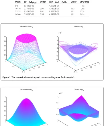
Table 1 Errors, convergence orders and CPU time for Example 1
Mesh u – uhL2() Order |{y – yh,σ–σh}|δ Order CPU time
8*8 5.5232E-02 - 4.0521E-01 - 5s
16*16 2.7731E-02 0.99 1.9822E-01 1.03 26s
32*32 1.3741E-02 1.01 9.8230E-02 1.01 127s
64*64 6.9009E-03 0.99 4.8929E-02 1.01 761s
Figure 1 The numerical controluhand corresponding error for Example 1.
Figure 2 The numerical stateyhand corresponding error for Example 1.
σ(x) = –∇y,
z(x) =sin(πx)sin(πx),
ω(x) =∇z,
u(x) =max,min{.,z},
Figure 3 The first component of numerical flux stateσhand corresponding error for Example 1.
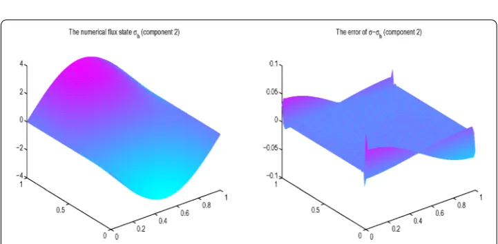
Figure 4 The second component of numerical flux stateσhand corresponding error for Example 1.
We can see that the solutions of this example areδ-independent. Table displays the errors and convergence orders with respect to the decreasing uniform mesh sizehfor the controluinL()-norm, the statesyandσin weighted norm. The main CPU time for the
computation excluding the mesh generation part is also listed. It uses no more than five cycles for the iteration algorithm. Figure shows the numerical solution and numerical error of the control when mesh sizeh= /, while the numerical solutions and errors of the state and flux state are presented in Figures -, respectively. It can be observed that the numerical results are in agreement with the analytical solutions very well.
Example For the second example, we consider a nonhomogeneous Dirichlet boundary problem. Let us takeσd= and consider Case IV withz=. The corresponding solutions of the optimal control problem are as follows:
y(x) =x( –x) +x( –x),
σ(x) = –∇y,
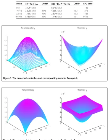
Table 2 Errors, convergence orders and CPU time for Example 2
Mesh u – uhL2() Order |{y – yh,σ–σh}|δ Order CPU time
8*8 7.1264E-02 - 9.5403E-02 - 8s
16*16 3.5255E-02 1.02 4.6587E-02 1.03 37s
32*32 1.7583E-02 1.00 2.3046E-02 1.02 172s
64*64 8.7859E-03 1.00 1.1465E-02 1.01 973s
Figure 5 The numerical controluhand corresponding error for Example 2.
Figure 6 The numerical stateyhand corresponding error for Example 2.
ω(x) =∇z–σ–σd –δ ,
u(x) =z,
where the source functionf and the desired statesydcan also be determined by (.) and (.), respectively.
Figure 7 The first component of numerical flux stateσhand corresponding error for Example 2.
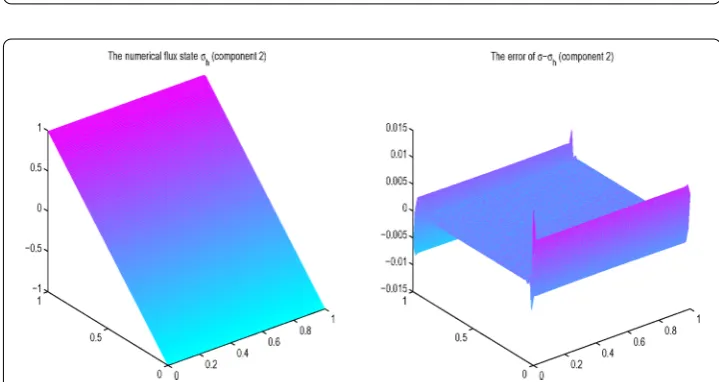
Figure 8 The second component of numerical flux stateσhand corresponding error for Example 2.
consistent with Theorem .. Besides, the numerical results are also well matched with the analytical solutions.
6 Concluding remarks
In this paper, we discuss a novel stabilized mixed finite element method for the approxi-mation of reaction-diffusion optimal control problem. Compared with our previous work, the novel method is more simple and easier to be implemented. It needs only one stabi-lization parameter but is still stable. Furthermore, low regularities for the state and ad-joint state variables are needed. Different cases of the admissible control set are discussed anda priorierror estimates are proved. Finally, numerical experiments are addressed to demonstrate the theoretical analysis. Most importantly, we should point that this novel stabilized mixed method is more competitive. It can easily be extended to solve optimal control problems governed by a bilinear state equation, the Stokes equation and so on.
Competing interests
Authors’ contributions
All authors read and approved the final manuscript.
Author details
1College of Science, China University of Petroleum, Qingdao, 266580, China.2College of Petroleum Engineering, China University of Petroleum, Qingdao, 266580, China.
Acknowledgements
This work was supported by the National Natural Science Foundation of China (Nos. 11201485, 11571367), the Promotive Research Fund for Excellent Young and Middle-aged Scientists of Shandong Province (No. BS2013NJ001), and the Fundamental Research Funds for the Central Universities (Nos. 14CX02217A, 15CX08004A, 15CX08011A). The first author was partially supported by the China Scholarship Council (No. 201506455014).
Received: 3 October 2015 Accepted: 12 January 2016
References
1. Ciarlet, PG: The Finite Element Method for Elliptic Problems. SIAM, Philadelphia (2002)
2. Brenner, SC, Scott, LR: The Mathematical Theory of Finite Element Methods. Springer, New York (2010) 3. Lions, JL: Optimal Control of Systems Governed by Partial Differential Equations. Springer, Berlin (1971) 4. Liu, W, Yan, N: Adaptive Finite Element Methods for Optimal Control Governed by PDEs. Series in Information and
Computational Science, vol. 41. Science Press, Beijing (2008)
5. Tiba, D: Lectures on the Optimal Control of Elliptic Equations. University of Jyväskylä Press, Jyväskylä (1995) 6. Hinze, M, Pinnau, R, Ulbrich, M, Ulbrich, S: Optimization with PDE Constraints. Springer, Berlin (2009)
7. Falk, FS: Approximation of a class of optimal control problems with order of convergence estimates. J. Math. Anal. Appl.44, 28-47 (1973)
8. Hinze, M: A variational discretization concept in control constrained optimization: the linear-quadratic case. Comput. Optim. Appl.30, 45-61 (2005)
9. Meyer, C, Rösch, A: Superconvergence properties of optimal control problems. SIAM J. Control Optim.43, 970-985 (2004)
10. Arada, N, Casas, E, Tröltzsch, F: Error estimates for the numerical approximation of a semilinear elliptic control problem. Comput. Optim. Appl.23, 201-229 (2002)
11. Chen, Y, Liu, W: Error estimates and superconvergence of mixed finite elements for quadratic optimal control. Int. J. Numer. Anal. Model.3, 311-321 (2006)
12. Yan, N, Zhou, Z: A RT mixed FEM/DG scheme for optimal control governed by convection diffusion equations. J. Sci. Comput.41, 273-299 (2009)
13. Chen, Y, Lu, Z: Error estimates of fully discrete mixed finite element methods for semilinear quadratic parabolic optimal control problem. Comput. Methods Appl. Mech. Eng.199, 1415-1423 (2010)
14. Zhou, J, Chen, Y, Dai, Y: Superconvergence of triangular mixed finite elements for optimal control problems with an integral constraint. Appl. Math. Comput.217, 2057-2066 (2010)
15. Fu, H, Rui, H: A characteristic-mixed finite element method for time-dependent convection-diffusion optimal control problem. Appl. Math. Comput.218, 3430-3440 (2011)
16. Gong, W, Yan, N: Mixed finite element method for Dirichlet boundary control problems governed by elliptic PDEs. SIAM J. Control Optim.49, 984-1014 (2011)
17. Raviart, PA, Thomas, JM: A mixed finite element method for 2nd order elliptic problems. In: Mathematical Aspects of Finite Element Methods. Lecture Notes in Mathematics, vol. 606, pp. 292-315. Springer, Berlin (1977)
18. Hughes, TJR, Franca, LP, Hulbert, G: A new finite element formulation for computational fluid dynamics: VIII. The Galerkin/least-squares method for advective-diffusive equations. Comput. Methods Appl. Mech. Eng.73, 173-189 (1989)
19. Franca, LP, Stenberg, R: Error analysis of Galerkin least squares methods for the elasticity equations. SIAM J. Numer. Anal.28, 1680-1697 (1991)
20. Franca, LP, Frey, SL, Hughes, TJR: Stabilized finite element methods: I. Application to the advective-diffusive model. Comput. Methods Appl. Mech. Eng.95, 253-276 (1992)
21. Franca, LP, Valentin, F: On an improved unusual stabilized finite element method for the advective-reactive-diffusive equation. Comput. Methods Appl. Mech. Eng.190, 1785-1800 (2000)
22. Fu, H, Rui, H, Hou, J, Li, H: A stabilized mixed finite element method for elliptic optimal control problems. J. Sci. Comput. (2015). doi:10.1007/s10915-015-0050-3.5