A priori error estimates for higher order variational discretization and mixed finite element methods of optimal control problems

(1)

R E S E A R C H

Open Access

A priori

error estimates for higher order

variational discretization and mixed finite

element methods of optimal control problems

Zuliang Lu

1,2*

, Yanping Chen

3

and Yunqing Huang

4

* Correspondence: zulianglux@126. com

1_{College of Civil Engineering and} Mechanics, Xiangtan University, Xiangtan 411105, PR China Full list of author information is available at the end of the article

Abstract

In this article, we investigatea priorierror estimates for the optimal control problems governed by elliptic equations using higher order variational discretization and mixed finite element methods. The state and the co-state are approximated by the orderkRaviart-Thomas mixed finite element spaces and the control is not discreted.

A priorierror estimates for the higher order variational discretization and mixed finite element approximation of control problems are obtained. Finally, we present some numerical examples which confirm our theoretical results.

Mathematics Subject Classification 1991: 49J20; 65N30.

Keywords:optimal control problems, variational discretization, mixed finite element methods,a priorierror estimates

1. Introduction

Optimal control problems governed by elliptic equations are important problems in engineering applications. Efficient numerical methods are critical for successful applica-tions of optimal control problems in such cases. Recently, the finite element method of optimal control problems plays an important role in numerical methods for these blems. Systematic introduction of the finite element method for optimal control pro-blems can be found in, for example, [1]. The finite element approximation of optimal control problem by piecewise constant functions is well investigated by Falk [2] and Geveci [3]. Arada et al. [4] discussed the discretization for semilinear elliptic optimal control problems. In [5], Malanowski discussed a constrained parabolic optimal control problems.

In many control problems, the objective functional contains gradient of the state variables. Thus accuracy of gradient is important in numerical approximation of the state equations. In the finite element community, mixed finite element methods should be used for discretization of the state equations in such cases. In computational opti-mal control problems, mixed finite element methods are not widely used in engineer-ing simulations. In particular there doesn’t seem to exist much work on theoretical analysis of mixed finite element approximation of optimal control problems in the lit-erature. More recently, we have done some preliminary work on sharp a posteriori

error estimates, error estimates and superconvergence of mixed finite element methods for optimal control problems (see, for example, [6-13]).

(2)

In [14], the author first presents the variational discretization concept for optimal control problems with control constraints, which implicitly utilizes the first order optimality conditions and the discretization of the state and adjoint equations for the discretization of the control instead of discretizing the space of admissible controls.

For 1≤p<∞andm, any nonnegative integer, let Wm,p(Ω) = {vÎLp(Ω); DbvÎ Lp

(Ω) if |b| ≤ m} denote the Sobolev spaces endowed with the norm vp_m_,_p=_|_β_|≤_mDβvp_Lp₍₎, and the semi-norm |v|

p m,p=

|β|=mDβv p

Lp₍₎. We set

W₀m,p() ={v∈Wm,p() :v|∂= 0}. For p = 2, we denote

Hm() =Wm,2(), H₀m() =W₀m,2(), and∥·∥m=∥·∥m,2, ∥·∥=∥·∥0,2.

In this article we derivea priorierror estimates for higher order variational discreti-zation and mixed finite element methods of quadratic optimal control problems.

We consider the following quadratic optimal control problems:

min u∈K⊂U

1

2p−pd 2

+1

2y−yd 2

+1 2u

2

(1:1)

subject to the state equation

divp=f +Bu, x∈, (1:2)

p=−A∇y, x∈, (1:3)

y= 0, x∈∂, (1:4)

where the bounded open setΩ⊂ℝ2, is a convex domain with the boundary∂Ω. We shall assume that pdÎ L2(Ω)2,yd Î L2(Ω), fÎ H1(Ω), andB is a continuous linear operator from U=L2(Ω) toH1(Ω). Furthermore, we assume the coefficient matrix A

(x) = (ai,j(x))2 × 2Î(W1,∞(Ω))2 × 2is a symmetric 2 × 2-matrix and there is a constant

c > 0 satisfying for any vector X∈R2, XAX≥cX2_R2. Here, Kdenotes the admissible

set of the control variable, defined by

K= ⎧ ⎨

⎩u∈U=L2() :

u≥0

⎫ ⎬

⎭. (1:5)

(3)

Now, we introduce the co-state elliptic equation

−div(A(∇z+p−p_d)) =y−yd, x∈, (1:6)

with the boundary condition

z= 0, x∈∂. (1:7)

The outline of this article is as follows. In Section 2, we construct the higher order variational discretization and mixed finite element approximation for optimal control problems governed by elliptic equations. Furthermore, we briefly state the definitions and properties of some interpolation operators. In Section 3, we derive a priorierror estimates for the higher order variational discretization and mixed finite element solu-tions of the optimal control problems. Numerical examples are presented in Section 4. Finally, we analyze the conclusion and the future studies in Section 5.

2. Variational discretization and mixed finite element methods

We shall now describe the variational discretization and mixed finite element approxi-mation of the optimal control problems (1.1)-(1.4). Let

V =H(div;) ={v∈(L2())2, divv∈L2()}, W=L2().

The Hilbert space Vis equipped with the following norm:

vdiv=vH(div;)=

v20,+divv20,

1/2 .

We recast (1.1)-(1.4) as the following weak form: find (p, y, u)Î V×W ×U such that

min u∈K⊂U

1

2p−pd 2

+1

2y−yd 2

+1 2u

2

(2:1)

(A−1p,v)−(y, divv) = 0, ∀v∈V, (2:2)

(divp,w) = (f +Bu,w), ∀w∈W. (2:3)

It is well known (see e.g., [15,16]) that the optimal control problem (2.1)-(2.3) has a solution (p, y,u), and that a triplet (p, y, u) is the solution of (2.1)-(2.3) if and only if there is a co-state (q, z)Î V×Wsuch that (p,y,q,z,u) satisfies the following optim-ality conditions:

(A−1p,v)−(y, divv) = 0, ∀v∈V, (2:4)

(divp,w) = (f +Bu,w), ∀w∈W, (2:5)

(A−1q,v)−(z, divv) =−(p−p_d,v), ∀v∈V, (2:6)

(divq,w) = (y−yd,w), ∀w∈W, (2:7)

(4)

where (·, ·)Uis the inner product of U,B* is the adjoint operator of B. In the rest of the article, we shall simply write the product as (·, ·) whenever no confusion should be caused.

Now, we will show that the control variable of the optimal control problem (2.4)-(2.8) can be infinitely smooth if the special constraint set Kdefined as (1.5).

Lemma 2.1. Let(p, y, q,z,u)Î (V×W)2×K be the solution of (2.4)-(2.8). Then we have

u= max0,B∗z−B∗z, (2:9)

where B∗z=B∗z/||denotes the integral average onΩof the function z.

Proof. If B∗z>0, then u=B∗z−B∗z and for anyvÎK

(u+B∗z,v−u) =

(u+B∗z)(v−u)

=

B∗zv−B∗z+B∗z

=B∗z

v≥0.

If B∗z≤0, thenu= -B*zand (u+B* z, v-u) = 0. Now, for the costate solutionz, since the solution of (2.8) is unique, then we have proved the Lemma.

From Lemma 3.1, we obtain the following regularity result for the control variable.

Lemma 2.2.Let(p, y, q,z, u)Î(V×W)2 ×K be the solution of (2.4)-(2.8).Assume that the data functions f, yd,pd,and the domainΩare infinitely smooth. Then the

con-trol function u∈C∞(¯).

Proof. By applying the regularity argument of elliptic problem (1.2)-(1.3), it is clear that y ÎH2(Ω), so thatpÎ H1(Ω). It follows from the costate Equation (1.6) and the assumption of yd, pd, we can obtain that z ÎH2(Ω). Using the relationship between the control and the costate u= max0,B∗z−B∗z, thenu ÎH2(Ω). ThusyÎ H4(Ω), p ÎH3(Ω). By repeating the above process, we can conclude that u∈C∞(¯).

Let Th be regular triangulation ofΩ. They are assumed to satisassociated with the

triangulationfy the angle condition which means that there is a positive constant C

such that for all T∈Th,C−1_h2

T≤ |T| ≤Ch2T, where |T| is the area of T, hTis the dia-meter of T and h= max hT. In addition C or cdenotes a general positive constant independent ofh.

Let Vh×Wh ⊂V×W denotes the Raviart-Thomas space [17] of the lowest order associated with the triangulation Th ofΩ.Pkdenotes the space of polynomials of total

degree at most k. Let V(T) ={v∈P2_k(T) +x·Pk(T)}, W(T) =Pk(T). We define

Vh :={vh∈V:∀T∈Th,vhT∈V(T)},

Wh:={wh ∈W:∀T∈Th,whT ∈W(T)}.

(5)

min uh∈K

1

2ph−pd 2

+1

2yh−yd 2

+1 2uh

2

(2:10)

(A−1p_h,vh)−(yh, divvh) = 0, ∀vh ∈Vh, (2:11)

(divp_h,wh) = (f+Buh,wh), ∀wh∈Wh. (2:12)

It is well known that the optimal control problem (2.10)-(2.12) again has a solution (ph,yh,uh), and that a triplet (ph,yh,uh) is the solution of (2.10)-(2.12) if and only if there is a co-state (qh, zh)ÎVh×Whsuch that (ph,yh,qh,zh, uh) satisfies the follow-ing optimality conditions:

(A−1p_h,vh)−(yh, divvh) = 0, ∀vh∈Vh, (2:13)

(divp_h,wh) = (f+Buh,wh), ∀wh∈Wh, (2:14)

(A−1q_h,vh)−(zh, divvh) =−(p_h−p_d,vh) ∀vh ∈Vh, (2:15)

(divq_h,wh) = (yh−yd,wh), ∀wh ∈Wh, (2:16)

(uh+B∗zh,u˜−uh)≥0, ∀˜u∈K. (2:17)

Let Ph:W®Whbethe orthogonalL2(Ω)-projection intoWhdefine by [18]:

(Phw−w,X) = 0, w∈W, X ∈Wh, (2:18)

which satisfies

Phw−w0,q≤Cwt,qht, 0≤t≤k+ 1, ifw∈W∩Wt,q(), (2:19)

Phw−w−r≤Cwthr+t, 0≤r, t≤k+ 1, ifw∈Ht(), (2:20)

(divvh,w−Phw) = 0, w∈W, vh∈Vh. (2:21)

Let πh:V®Vhbe the Raviart-Thomas projection [19], which satisfies

(div(πhv−v),wh) = 0, v∈V, w∈Wh, (2:22)

πhv−v0,q≤Cvt,qht, 1/q<t≤k+ 1, ifv∈V∩Wt,q()2, (2:23)

div(_πhv−v)₀≤Cdivv_tht, 0≤t≤k+ 1, ifv∈V∩Ht(div;). (2:24)

We have the commuting diagram property [20]

div◦πh=Ph◦div :V →Wh and div(I−πh)V⊥Wh, (2:25)

(6)

3. A priorierror estimates

In the rest of the article, we shall use some intermediate variables. For any control function ũÎK, we first define the state solution (p(ũ),y(ũ),q(ũ),z(ũ)) associated with

ũthat satisfies

(A−1p(u˜),v)−(y(u˜), divv) = 0, ∀v∈V, (3:1)

(divp(u˜),w) = (f+Bu˜,w), ∀w∈W, (3:2)

(A−1q(u˜),v)−(z(u˜), divv) =−(p(u˜)−p_d,v), ∀v∈V, (3:3)

(divq(u˜),w) = (y(u˜)−yd,w), ∀w∈W. (3:4)

Correspondingly, we define the discrete state solution (ph(ũ),yh(ũ),qh(ũ),zh(ũ)) asso-ciated withũÎKthat satisfies

(A−1p_h(u˜),vh)−(yh(u˜), divvh) = 0, ∀vh∈Vh, (3:5)

(divp_h(u˜),wh) = (f+Bu˜,wh), ∀wh∈Wh, (3:6)

(A−1q_h(u˜),vh)−(zh(u˜), divvh) =−(p_h(u˜)−p_d,vh), ∀vh∈Vh, (3:7)

(divq_h(u˜),wh) = (yh(u˜)−yd,wh), ∀wh∈Wh. (3:8)

We define another discrete state solution (pˆ_h(u),ˆzh(u)) that satisfies

(A−1qˆh(u˜),vh)−(zˆh(u˜), divvh) =−(p−pd,vh), ∀vh∈Vh, (3:9)

(divqˆ_h(u˜),wh) = (y−yd,wh), ∀wh ∈Wh. (3:10)

Thus, as we defined, the exact solution and its approximation can be written in the following way:

(p,y,q,z) = (p(u),y(u),q(u),z(u)), (p_h,yh,q_h,zh) = (p_h(uh),yh(uh),q_h(uh),zh(uh)).

Combining Lemma 2.1 in [19] and (2.19), we obtain the following technical results:

Lemma 3.1.LetωÎV,ÎL2(Ω)2,andψÎL2(Ω).IfτÎ Whsatisfies

(A−1_ω_,_v_h)₋₍_τ_{, div}_v_{h) = (}_ϕ_,_v_h),_∀_v h∈Vh, (divω,wh) = (ψ,wh), ∀wh∈Wh,

then, there exists a constant C such that

τ0≤C

hω0+hdivω₀+ϕ0+ψ0

, (3:11)

for h sufficiently small.

Now we choseũ=uin (3.5)-(3.8), then we set some intermediate errors:

(7)

To analyze the intermediate errors, let us first note the following error equations from (2.4), (2.5), (3.5) and (3.6) with the choiceũ=u:

(A−1ε1,vh)−(e1, divvh) = 0, ∀vh∈Vh, (3:13)

(divε1,wh) = 0, ∀wh∈Wh. (3:14)

By (2.18)-(2.24) and Lemma 3.1, we can establish the following error estimates:

Theorem 3.1. Assume that yÎ Hk+3(Ω). If h is sufficiently small, there is a positive constant C independent of h such that

y−yh(u)₀≤Chk+1, (3:15)

p−p_h(u)₀≤Chk+1, (3:16)

p−p_h(u)_div≤Chk+1. (3:17)

Proof. Letτ=Phy-yh(u) ands=πhp-ph(u). Rewrite (3.13) and (3.14) in the form (A−1ε1,vh)−(τ, divvh) = 0, ∀vh∈Vh, (3:18)

(divε1,wh) = 0, ∀wh∈Wh. (3:19)

It follows from Lemma 3.1 that

τ0≤C

hε10+hdivε1₀

. (3:20)

By using (2.19) that

e10=y−yh(u)₀ =Phy−y₀+τ0

≤Chε10+hdivε1₀+hk+1y_k₊₁

.

(3:21)

If we now again rewrite (3.13) and (3.14) as

(A−1_σ_,_v

h)−(τ, divvh) = (A−1(πhp−p),vh), ∀vh∈Vh, (3:22)

(divσ,wh) = 0, ∀wh∈Wh. (3:23)

Using the standard stability results of mixed finite element methods in [21], we establish the following results:

σdiv≤Cπhp−p₀+e10

≤C

hk+1y_k₊₂+e10

. (3:24)

(8)

ε10≤Cπhp−p₀+σ0

≤Chk+1y_k₊₂+e10

, (3:25)

and

divε1₀≤Cdiv(πhp−p)₀+divσ₀

=CPh◦divp−divp₀+divσ₀

≤C

hk+1y_k₊₃+e10

,

(3:26)

when substituted into (3.21), which yields the estimate

e10≤C

he10+hk+1y_k₊₁

. (3:27)

Then (3.27) implies (3.15) holds if his small enough. Applying (3.27) to (3.25) and (3.26) shows that (3.16) and (3.17) also hold.

With the intermediate errors, we decompose the errors as follows

p−p_h=p−p_h(u) +p_h(u)−p_h:=ε1+1, (3:28)

y−yh=y−yh(u) +yh(u)−yh:=e1+r1. (3:29)

From (2.13), (2.14), (3.5) and (3.6), we have

(A−11,vh)−(r1, divvh) = 0, ∀vh∈Vh, (3:30)

(div1,wh) = (B(u−uh),wh), ∀wh∈Wh. (3:31)

The assumption that AÎ L∞(Ω;ℝ2 × 2) implies that it is bounded that the inverse operator of the map {1,r1}:ℝ3 ®V×Wdefined by the above saddle-point problem

[21]:

1div+r10≤Cu−uh0, (3:32)

where the continuity of the linear operator Bhas been used. Now we are able to derive our main results.

Theorem 3.2.Let(p,y, q,z,u)Î (V×W)2 ×K and(ph,yh,qh,zh,uh)Î(Vh×Wh)2 ×K be the solutions of(2.4)-(2.8)and (2.13)-(2.17),respectively. We assume thaty, zÎ Hk+3(Ω).

Then, we have

u−uh0≤Chk+1, (3:33)

p−p_h_div+y−yh₀≤Chk+1, (3:34)

q−q_h_div+z−zh0≤Chk+1. (3:35)

Proof. We chooseũ=uhin (2.8) andũ=uin (2.17) to get that

(9)

and

(uh+B∗zh,u−uh)≥0. (3:37)

Then we have

u−uh2≤(B∗zh−B∗z,u−uh)

= (B∗ˆzh(u)−B∗z,u−uh) + (B∗zh−B∗zˆh(u),u−uh).

(3:38)

Moreover, theδ-Caunchy inequality leads that

(B∗zˆh(u)−B∗z,u−uh)≤Cˆzh(u)−z· u−uh

≤Czˆh(u)−z 2

+Cδu−uh2,

(3:39)

where δis an arbitrary positive number. From (3.30)-(3.31), (2.15)-(2.16) and (3.9)-(3.10), we obtain the following equations:

(A−1(p_h−p_h(u)),vh)−(yh−yh(u), divvh) = 0, ∀vh∈Vh, (3:40)

(div(p_h−p_h(u)),wh) = (B(u−uh),wh), ∀wh∈Wh, (3:41)

(A−1(qˆ_h(u)−q_h),vh)−(zˆh(u)−zh, divvh) =−(p−ph,vh), ∀vh ∈Vh, (3:42)

(div(qˆ_h(u)−q_h),wh) = (y−yh,wh), ∀wh∈Wh. (3:43)

By applying the above error equations, we obtain

(B∗zh−B∗zˆh(u),u−uh) = (zh− ˆzh(u),B(u−uh)) = (div(p_h−p_h(u)),zh− ˆzh(u))

= (A−1(qˆ_h(u)−q_h),p_h−p_h(u)) + (p−p_h,p_h−p_h(u)) = (yh−yh(u), div(qˆh(u)−qh) + (p−ph,ph−ph(u)) = (y−yh,yh−yh(u)) + (p−ph,ph−ph(u))

= (y−yh,y−yh(u)) + (p−p_h,p−p_h(u))−y−yh2−p−ph 2

=y−yh·y−yh(u)+p−ph·p−ph(u)−y−yh 2

−p−p_h2

≤Cy−yh(u)2+Cp−p_h(u)2− 1

2y−yh 2

−1

2p−ph 2

.

(3:44)

From (3.38), (3.39), and (3.44), we derive that

u−uh2+y−yh 2

+p−ph 2

≤Cy−yh(u)2+Cp−p_h(u)2+Cz− ˆzh(u)2. (3:45)

Note that zˆh(u),qˆ_h(u) are the mixed finite element approximation ofz,q, using the results of [22], we have

(10)

From the Theorem 3.1, (3.45), and (3.46), we obtain

u−uh+y−yh+p−ph≤Chk+1, (3:47)

then we derive (3.33). By using (3.42) and (3.43) and the stability results of mixed finite element methods [21], we have

qˆ_h(u)−q_h_div+ˆzh(u)−zh≤Cp−ph+Cy−yh. (3:48)

Combining (3.46)-(3.48), we derive the following result

q−q_h_div+z−zh ≤Chk+1. (3:49)

From (3.17), (3.32), and (3.47), it is easy to see that

p−p_h_div≤Chk+1. (3:50)

Then we derive the results (3.34) and (3.35).

4. Numerical tests

In this section, we are going to validate the a priorierror estimates for the error in the control, state, and co-state numerically. The optimization problems were dealt numeri-cally with codes developed based on AFEPACK. The package is freely available and the details can be found at [23].

In our numerical examples, we consider the following optimal control problems:

min u∈K

1

2p−pd 2

+1

2y−yd 2

+1 2u

2

(4:1)

divp=Bu+f, p=−A∇y, x∈, y|_∂= 0, (4:2)

divq=y−yd, q=−A(∇z+p−p_d), x∈, z|_∂= 0. (4:3)

In our examples, we choose the domain Ω= [0, 1] × [0, 1] andA=B=I. We pre-sent below two examples to illustrate the theoretical results of the optimal control pro-blems. The convergence order is computed by the following formula: order

log(Ei/Ei+1) log(hi/hi+1)

, wherei responds to the spatial partition, and Ei denotes the for the

state, costate and control approximation.

Example 1. In this example we set the other known functions as follows:

y= 2 sinπx1sinπx2,

z=−sinπx1sinπx2,

q= (πcosπx1sinπx2,πcosπx2sinπx1),

yd= (1 +π2)y, p=pd=−2q,

f = 2π2y−u,

u= max(z¯, 0)−z.

In this numerical implementation, the error ∥u- uh∥0, ∥p - ph∥div, ∥y- yh∥0, ∥ q

-qh∥div, and∥z - zh∥0 obtained on RT0 mixed finite element approximation and RT1

(11)

and 4. The theoretical results can be observed clearly from the data. The profile of the

numerical solution is plotted in Figures 1 and 2.

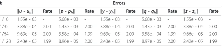
Example 2. In this example we set the other known functions as follows:

y= (x1+x2) sinπx1sinπx2,

z=−(x1+x2) sinπx1sinπx2,

u= max(z¯, 0)−z, p=p_d=−q,

f = 2π2sinπx1sinπx2(x1+x2) + cosπx1sinπx2−u,

q= (πcosπx1sinπx2+ sinπx1sinπx2,πcosπx2sinπx1+ sinπx1sinπx2),

yd=y+ 2π2sinπx1cosπx2(x1+x2)−2πcosπx1sinπx2−2πsinπx1cosπx2.

[image:11.595.116.480.102.177.2]

The example obviously indicates that the error estimates remains in output data. From the error data in the two examples, it can be seen that the priori error estimates that we have mentioned is exact.

Table 1 The numerical errors on RT0 mixed finite element for state function

h Errors

[image:11.595.117.478.235.313.2]

∥u-uh∥ Rate ∥p-ph∥ Rate ∥y-yh∥ Rate ∥q-qh∥ Rate ∥z-zh∥ Rate 1/16 3.63e - 02 - 3.25e - 01 - 7.24e - 02 - 1.63e - 01 - 3.63e - 02 -1/32 1.80e - 02 1.01 1.62e - 01 1.00 3.63e - 02 0.99 8.12e - 02 1.01 1.80e - 02 1.01 1/64 9.06e - 03 0.99 8.13e - 02 0.99 1.78e - 02 1.03 4.07e - 02 1.00 9.06e - 03 0.99 1/128 4.48e - 03 1.01 4.03e - 02 1.01 8.87e - 03 1.01 2.05e - 02 0.99 4.48e - 03 1.01

Table 2 The numerical errors on RT1 mixed finite element for state function

h Errors

Table 3 The numerical error on RT0 mixed finite element for state function

h Errors

Table 4 The numerical error on RT1 mixed finite element for state function

h Errors

[image:11.595.117.478.360.436.2] [image:11.595.118.479.658.733.2]

(12)

5. Conclusion and future works

The present article discussed the higher order variational discretization and mixed finite element methods for the optimal control problems governed by elliptic equa-tions. We have obtained some error estimate results for both the state, the co-state and the control approximation with convergence order hk+1. The priori error estimates

0 0.5

1 0

0.5

1 0

[image:12.595.119.480.87.349.2]

5 10 15 20

Figure 1The profile of the control solutionuon the 64 × 64 mesh grids.

0

0.2 0.4

0.6 0.8

1

0 0.2 0.4 0.6 0.8 1 0 0.5 1 1.5

[image:12.595.119.480.478.715.2]

(13)

for the elliptic optimal control problems by variational discretization and mixed finite element methods seem to be new.

In our future study, we shall use the variational discretization and mixed finite ele-ment method to deal with the optimal control problems governed by nonlinear para-bolic equations and convex boundary control problems. Furthermore, we shall consider a priori error estimates and superconvergence of optimal control problems governed by nonlinear parabolic equations or convex boundary control problems.

Acknowledgements

The authors express their thanks to the referees for their helpful suggestions, which led to improvements of the presentation. Zuliang Lu was by the supported National Science Foundation of China (11126329) and China Postdoctoral Science Foundation (2011M500968). Yanping Chen was supported by the Guangdong Province Universities and Colleges Pearl River Scholar Funded Scheme (2008), National Science Foundation of China (10971074), and Specialized Research Fund for the Doctoral Program of Higher Education (20114407110009). Yunqing Huang was supported by the NSFC Key Project (11031006) and Hunan Provincial NSF Project (10JJ7001).

Author details

1_{College of Civil Engineering and Mechanics, Xiangtan University, Xiangtan 411105, PR China}2_{School of Mathematics} and Statistics, Chongqing Three Gorges University, Chongqing 404000, PR China3_{School of Mathematical Sciences,} South China Normal University, Guangzhou 510631, PR China4_{Hunan Key Laboratory for Computation and Simulation} in Science and Engineering, Department of Mathematics, Xiangtan University, Xiangtan 411105, Hunan, PR China

Authors’contributions

ZL carried out the molecular genetic studies, participated in the sequence alignment and drafted the manuscript. YC participated in the design of the study and performed the statistical analysis. YH conceived of the study, and participated in its design and coordination. All authors read and approved the final manuscript.

Competing interests

The authors declare that they have no competing interests.

Received: 11 January 2012 Accepted: 20 April 2012 Published: 20 April 2012

References

1. Lions, JL: Optimal Control of Systems Governed by Partial Differential Equtions. Springer, Berlin (1971)

2. Falk, FS: Approximation of a class of optimal control problems with order of convergence estimates. J Math Anal Appl.

44, 28–47 (1973)

3. Geveci, T: On the approximation of the solution of an optimal control problem governed by an elliptic equation. RAIRO Numer Anal.13, 313–328 (1979)

4. Arada, N, Casas, E, Tröltzsch, F: Error estimates for the numerical approximation of a semilinear elliptic control problem. Comput Optim Appl.23, 201–229 (2002)

5. Malanowski, K: Convergence of approximation vs.regularity of solutions for convex control constrained optimal control systems. Appl Math Optim.34, 134–156 (1992)

6. Chen, Y: Superconvergence of optimal control problems by rectangular mixed finite element methods. Math Comput.

77, 1269–1291 (2008)

7. Chen, Y, Dai, L, Lu, Z: Superconvergence of quadratic optimal control problems by triangular mixed finite elements. Adv Appl Math Mech.75, 881–898 (2009)

8. Chen, Y, Liu, WB: Error estimates and superconvergence of mixed finite elements for quadratic optimal control. Int J Numer Anal Model.3, 311_–321 (2006)

9. Chen, Y, Lu, Z: Error estimates for parabolic optimal control problem by fully discrete mixed finite element methods. Finite Elem Anal Des.46, 957_–965 (2010)

10. Chen, Y, Lu, Z: Error estimates of fully discrete mixed finite element methods for semilinear quadratic parabolic optimal control problems. Comput Methods Appl Mech Eng.199, 1415_–1423 (2010)

11. Lu, Z, Chen, Y, Zhang, H: A priori error estimates of mixed finite element methods for nonlinear quadratic optimal control problems. Lobachevskii J Math.29, 164_–174 (2008)

12. Lu, Z, Chen, Y: A posteriori error estimates of triangular mixed finite element methods for semilinear optimal control problems. Adv Appl Math Mech.1, 242–256 (2009)

13. Lu, Z, Chen, Y:L∞-error estimates of triangular mixed finite element methods for optimal control problem govern by semilinear elliptic equation. Numer Anal Appl.12, 74–86 (2009)

14. Hinze, M: A variational discretization concept in control constrained optimization: the linear-quadratic case. J Comput Optim Appl.30, 45–63 (2010)

15. Liu, WB, Yan, NN: A posteriori error estimates for distributed convex optimal control problems. Numer Math.101, 1_–27 (2005)

16. Liu, WB, Yan, NN: A posteriori error estimates for control problems governed by nonlinear elliptic equation. Adv Comput Math.15, 285–309 (2001)

17. Grisvard, P: Elliptic Problems in Nonsmooth Domains. Pitman, London (1985)

(14)

19. Miliner, FA: Mixed finite element methods for quasilinear second-order elliptic problems. Math Comput.44, 303–320 (1985)

20. Carstensen, C: A posteriori error estimate for the mixed finite element method. Math Comput.66, 465–476 (1997) 21. Brezzi, F, Fortin, M: Mixed and Hybrid Finite Element Methods. Springer, Berlin (1991)

22. Douglas, J Jr, Roberts, JE: Global estimates for mixed finite element methods for second order elliptic problems. Numer Funct Anal Optim.22, 953_–972 (2001)

23. Li, R, Liu, WB:http://www.math.zju.edu.cn/matlkw/afepack.html

doi:10.1186/1029-242X-2012-95

Cite this article as:Luet al.:A priorierror estimates for higher order variational discretization and mixed finite element methods of optimal control problems.Journal of Inequalities and Applications20122012:95.

Submit your manuscript to a

journal and benefi t from:

7Convenient online submission

7Rigorous peer review

7Immediate publication on acceptance

7Open access: articles freely available online

7High visibility within the fi eld

7Retaining the copyright to your article