Optimum Values of the Bandwidth of the Optical and Electrical Filters for a System
of High Mode Coupling Optical Fibers
Suad M. Abuzariba, Fathi Abubrig, Mohamed Delfag Physics Department, Misurata University
2478, Misurata, Libya
ABSTRACT: All-optical long-haul network in a rapid development to increase the optical communication systems capacity. As a point in this direction we report the optimum values of the bandwidth of the optical for a system of high mode coupling optical fibers using DPSK modulation format for the input signal with considering the impairments CD, PMD, PDL, and the noise. Furthermore, we did get the optimum electrical filters bandwidth as well.
Keywords: Bit Error Rate, Optical Filter, Electrical Filter
Received:
© 2013 DLINE. All rights reserved
1. Introduction
With increasing the bit rates, as the main point for developing the optical fiber communications systems, we need to develop each device in the optical fiber systems. Highly sensitive direct-detection receivers are the most important device in the designing of high-speed communication systems. In fact, optically preamplifier receivers show the best performance when employing match optical filters [1, 2]. On the other hand, nonmatched filters are commonly used these days. Fabry-Perot filters are the most ones that used today in order to maximize receiver sensitivity [3-5]. In order to maximize receiver sensitivity, optimum optical filter bandwidths ranging from 0.9 to 8 times the data rate have been proposed for nonreturn-to-zero (NRZ), ON-OFF kenning (OOK) transmission [5-7]. In this work, we present optimum optical filter bandwidth for Fabry-Perot filters for return-to-zero (RZ), Differential phase shift keying (DPSK) with considering the impairments chromatic disperstion (CD), polarization mode dispartion (PMD), polarization dependent loss (PDL), and the noise. Furthermore, we did get the optimum electrical filters bandwidth for the a fifth-order Bessel type.
2. The System Modeling
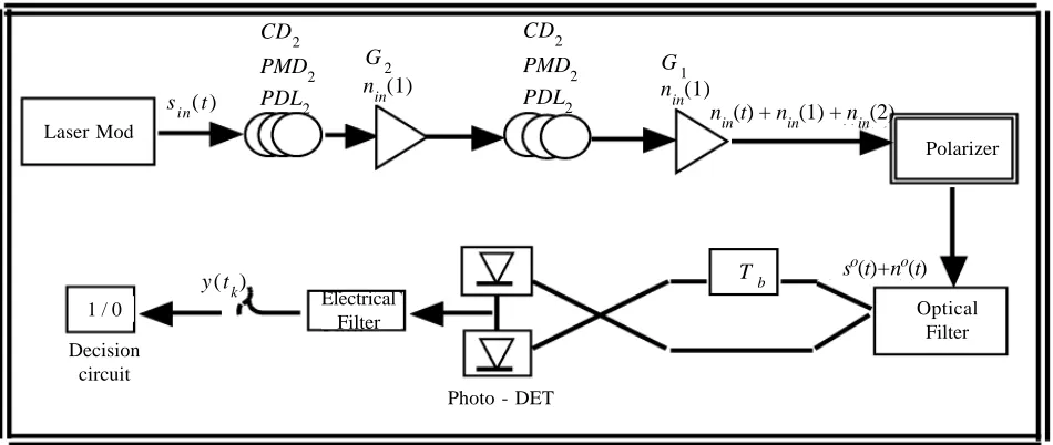
In our modeling system, figure (1) for DPSK, the optical signal sin t is launched into the fiber system with two lumped chromatic dispersion (CD1 and CD2), lumped PMD (PMD1 and PMD2), and lumped PDL (PDL1 and PDL2) in linear regime. Then it is amplified by a flat gain amplifier G. This amplifier added amplified spontaneous emission (ASE) noise. The normalized ASE
G − 1
G hv, where nsp N0 = nsp
noise is considered as additive white Gaussian noise nin t with two-sided power spectral density
≥ 1 is the spontaneous-emission or population inversion parameter and hv is the photon energy. We consider that G >> 1 so that N0 = nsp hv [8]. ASE noise from the flat gain amplifier G is partially polarized due to the PDL [9] then the signal is optically filtered using an optical filter. The optical filter is followed by photo detector. Finally the detected current is electrically filtered by the post detection filter and sampled at the time t.
The instantaneous current at the decision circuit can be written as
y t,t = <Eout t, t Eout t> + <Eout t Eout t, t> / 2
t = 0 (OOK), t = Tb (DPSK)
Using Fourier transform E t = 1 dt e−iωt E (ω), the instantaneous current is 2π
y t, t = 1
2πdω dω e i ω−ωt
eiωt + e−iωt Hrω−ω Ho*ω Hoω × < Eoutω Eoutω>
We are dealing with two sections of PMD, two sections of PDL and two noises, so the output field has the form
Eoutω = ei Ψ CD L 1ω + Ψ
CD L2 T α
2 T τ2 ,ω T α1 T τ1 ,ω
Einω >= ei ΨL 2 CD
ω T α
2 T τ2 ,ω e1 ω > (n)
Where e1 (n) and e2 (n) representing ASE noise optical fields.
The PMD Jones matrix has the form, T τ1 ,ω = exp (−i1
2ωτj . σ ), PDL Jones matrix is T αj = exp (− αj/ 2) exp (αj. σ) / 2 and the chromatic dispersion up to the 3rd order is Ψj = Lj [1
2β2ω
2
+ (1 6) β3ω
3
]. j denoted to the number of the section (j =1, 2).
Eoutω >= S1 + S2 + S3, S1 = ei ΨL1ω + ΨL2T α
2 T τ2 ,ω T α1 T τ1 ,ω , Einω > CD
S2 = ei ΨL2ω T α2 T τ2 ,ω, e1ω >
CD n
and S3 = e2nω >
For the critical expression <Eoutω Eoutω> we have nine distinct terms a
<Eoutω Eoutω> = S1 * S1 + S2 * S2 + S3 * S3 + S1 * S2 + S2 * S1 + S1 * S3 + S3 * S1 + S2 * S3 + S3 * S2 In order to proceed with the noise fields averaging, we introduce the following short hand notation
f ω, ω, t,t = 1
2π e i ω−ω t
eiωt + e−iωt Hrω−ω Ho*ω Hoω Also, we introduce a super noise field vector (depending on the noise fields dimensions)
Nω >= e1 ω >
e2 ω >
(n)
Furthermore, by discarding the noise expressions in the last eight terms of <Eoutω Eoutω> we can introduce a ket-vector
< b ω = dω f (ω, ω, t,t) S1* S2 dω f (ω, ω, t,t) S1* S3 bω >= dω f (ω, ω, t,t) S2 S1
dω f (ω, ω, t,t) S3 S1
* *
On the other hand we will combine the terms S1* S2 and S1* S3 to introduce the bra-vector
Finally, we introduce the square block matrix Q containing the terms S2 *S2
,
S3 *S3,
S3 *S3and S3 *S2 asdω f (ω, ω, t,t) S2 S2 dω f (ω, ω, t,t) S2 S3
dω f (ω, ω, t,t) S2 S2 dω f (ω, ω, t,t) S2 S3
*
* *
*
Q =
(1)
(2)
(3)
CD
For simplicity we will rewrite equation (5.4) as following
CD
(4)
(5.a)
(5.b)
(5.c)
(6)
(n) (7)
(8.a)
(8.b)
With the new vectors; the ket-vector N ω > , the bra-vector < b ω, the ket-vector b ω > and the square matrix Q, we can rewrite the instantaneous detecting current at the decision circuit as
y t, t = <N Q N> + <b N> + <N b> + dω dω f (ω, ω, t, t) S1 S1
1 2π
*
In fact, this equation is just another photo to equation (5.2). Mathematically, y t, tis a physical variable which is a function of complex Gaussian variable, in this case we can get the moment generation function as following: for a physical variable ξ which is defined in a quadratic form as ξ = c + λw* w + b* w + bw*and w = x + iy is a complex Gaussian variable. Then ξ = c + λx2 + y2 + 2xRe b + 2y Im(b) and its characteristic function is
eisξ =− ∞∞ dx PG x− ∞∞ dy PG y eisξ =
1 −σ 2 λis
1
e[isc σ 2
b s
1 −σ 2 λis]
Using inverse Fourier transform, from the characteristic function we can get the probability density function as
p ξ = − ∞∞ ds e−isξ< eisξ > = 1)
2π
( ds e−is(ξ − c)
− ∞ ∞
1 −σ 2 λis
1
e[isc
σ 2b s
1 −σ λis
]
For M complex random i.i.d. Gaussian variable we have ξ = c +M diag λj wj wj + bj wj + wj bj, The moment generation func-j = 1
∗ ∗ ∗
tion is
M j = 1
1 −σ 2 λj is
1
e[
σ 2bj s2
1 −σ 2 λ is]
2
j
Ψt kt =
and the probability density function is
p ξ = 1)
2π
( ds e−is(ξ − c) − ∞
∞ M
j = 1
1 −σ 2 λj is
1
e[−
σ 2bj s2
1 −σ λ is
]
2
j
Now if compare ξ with our current y we find that
c = yss = dω dω f ω, ω, t,t S1* S1 ξ− c = In =M diag λj wj∗ wj + bj∗ wj + w∗j bj
j = 1 =< N Q N> + <b N> + <N b>
With the known λj and by replacing is → s and using the inverse Laplace transform we have
ρ yss + In = 1 u0 + i∞ 2iπ
( )
u0− i∞
ds e− s(Ι n )
M
j = 1 1 −σ 2 λ j is
1
e [σ
bj s
1 −σ 2 λ j s]
2 22
σ 2max {λ j }
1
− < u0 <
σ 2max {λ j }
1 +
Here λj , λj stands for the positive and negative λj, respectively. Therefore, to evaluate the probability density function as a function of the whole detecting current (y = yss + In) we need to get the values of the integration as a function of the part related to noise (In); the noise-noise beating and the signal-noise beating.
For moment generation function given in equation (5.14), we can rewrite the probability density function as
+ −
ρy ς = 1 2iπ th
u0 + i∞
u0− i∞
ds Ψt s e− s ς,
σ 2max {λ j }
1
− < u0 <
σ 2max {λ j }
1 + k
P yss < yth = − ∞
y thρ
y ς dς =
th − ∞
∞
ρy ς u(yth
−
ς)dς thwhere yth is the detection threshold, and u (x) is a unit step function. Using the inverse Laplace transform we get
P {yss < yth }= 1 2iπ
u0 + i∞
u0− i∞
Ψt k s
s e
− sy thds ,
σ 2max λ
j }
1
− < u0 < 0
(10) 2 2 (11) 2 2 2 (12) (13)
2 (14)
(15)
(16)
(17)
(18)
where the restriction on the u0 range is necessary for the convergence of the inner integral in the last two equations.The right-hand tail probability can be evaluated in similar manners
P yss < yth =− ∞y th
ρy ς dς =
th − ∞
∞
ρy ς u(yth −ς)dς th
P {yss > yth}= 1 2iπ
u0 + i∞
u0− i∞ Ψt k s(
− ∞ ∞
u(ς −yth )e− s ς, dς ) ds
P {yss > yth}= − 1 2iπ
u0 + i∞
u0− i∞
Ψt k s s e
− sy thds ,
σ 2max λ
j }
1 + 0 < u0 <
Duo to the independency of the line integral of an analytic function and the integration path, we can rewrite both the left-hand tail and the right-hand tail as
P yss < yth = − 1 2iπ c−
Ψt k s s e
− sy thds , P yss > yth = 1
2iπ c + Ψt k s
s e
− sy thds.
The integration contours c± are conveniently chosen to closely approximate the paths of steepest descent passing through the saddle points u0 of the integrands on the real x-axis.
Ψt k s
s e
− sy
th=e Φ (s)
Let us take a look to the integrands in the last two equations; we can write, tk , taking the logarithmic fu-nction of the both sides gives
Φt
s = log Ψt s − log s − syth
k k
Substitute the value of Ψt t from equation (5.14) gives
The roots of this equation are the saddle points u0 and u0 . These two roots (saddle points) can be found by using a numerical method. Using Newton’s method we can get the saddle points, the paths of steepest descent c± are well approximated by
k
− +
parabolas of the form: s = u0 + 1 2kv
2
+ iv k =
± Φ′′′tk u0±
3Φ′′tk u0± whereΦ′′′tk u0
±
is the third derivative of Φ tk u0±. In order to
eval-uate the probabilities given in equations (5.24.a.), (5.24.b), we rewrite those two equations as
P yss < yth =π1 Re {eΦ 0 ∞
k t ( u +
0 + 1 2kv + iv) 2
(1 − ikv)}
P yss > yth = −1
π 0∞ Re {eΦtk( u +0
− 1 2kv
+ iv) 2
(1 − ikv)}
These two integrations are evaluated by the trapezoidal rule to get
P yss > yth ≅−∆γ
π n =1
∞ [ 1
2f 0 + f (n∆γ)] For the Zero bit, and for the One bit we have
P yss < yth ≅−∆γ
π n =1
∞ [ 1
2 f 0 + f (n∆γ)]
where f γ = Re {eΦtk( u +0
- 1
2kv
+ iv) 2
1 − ikv} and the initial step size is ∆γ = 1
2Φ′′tk u0± The sum of f (n∆γ) can be stopped when f (n∆γ) becomes negligible and halving the step size until the result is stabilized in desired accuracy. The bit error rate can be obtained using the form [8, 10]
± 1 2π i c ±
Ψt k s
s e
− sy thds BERy tk =
th
BER =k = 0N−1BERth (tk) / N
and tk = t0+ kTb. To include the intersymbol interference, we used a 32-bit sequence (16-Zeros and 16-Ones). Hence, the probability of error in Zeros bits is P0 =
P0 tk k = 0
15
16 . Similarly, the probability of error in Ones bits is P1 =
P1 tk k = 0
16
probability of error (assuming bits One and Zero are sent with equal probability) is BER =
The total
P0 + P1
2 . When the system input has a on-off keying (OOK) modulation format, the sequence an has taken 25-bit de Bruijn sequence [8, 10-12], i.e., 0000 0111 0111 1100 1011 0101 0011 0001. Repetition of this sequence yields all possible configurations of a 5-bit string from 00000 to 11111 [8,10]. For the system with a balanced DPSK receiver shown in Figure (5.4.b), ai = (∈{ei0, eiπ}) is determined by requiring the received codes at sampling instants tk ( tk = t0 + kTb, k = 0,..., N −1, normalized as “0” or “1” with no signal distortion, form a de Bruijn sequence. Different signal pulse shapes mean different spectral bandwidth, while different modulations can result in different correlations between adjacent signal bits and thus leads to different signal spectral distributions. The first-order PMD (i.e., DGD) causes the difference in arrival times of the two orthogonal modes of optical signal and leads to pulse broadening in time domain. Thus the RZ signal should be more tolerant to the PMD-induced intersymbol interference (ISI) than the NRZ signal, because the PMD effect on the RZ signal can be viewed as the increment of its duty cycle. Furthermore, RZ-DPSK has lower peak power and constant pulse amplitude which reduces the effect of fiber nonlinearity. Therefore, we used RZ-DPSK as input signal. The amplitude of the input signal sin t can be assumed to be a periodic repetition of signal dt =i = 0N−1ai p (t − iTb)with period NTb, sin t = sin t =
ai and determines the logic value of the ith bit. When N is large enough st is a pseudorandom signal. In this case we can use ∞
n = −∞d (t − nNTb) Here p(t) determines the elementary input pulse shape
a mathematical tractability with physical properties close to the real situations. This amplitude is n = −∞
∞ d t − nNT
b ≡l = −∞ ∞ st =
sl e2iπ lt/(NT )b, where sl =P( fl )
NTb Al , Al=m = 0 N−1
e-2iπ ml/N, with P f
l = dt p t e−
2iπ fl t/N, f
l = l / NTb
.
0
Tb
In the low-pass configuration, pt
is the elementary input pulse shape. We consider a raised cosine as input pulse. The raised cosine pulse [10] is given as pt =
, where Eb is the optical energy per transmitted bit. Due to its periodicity, the input signal sin t can be expa-2Eb Tb cos cos2
2 π t Tb π
nded in Fourier series as sin t = sin t ps >=
input signal are polarized in the same direction represented by a constant unit vector ps >= [x, y]T in 2D Jones space.
When the overall impulse response of the pre- and postdetection filters at the receiver has finite time duration T0, then the value of the sample y(tk) is solely determined by the values that the input waveform of the optical filter takes on in the time interval (tk − T0, tk). Real filters, practically, have finite impulse responses. However, theoretical filters may not have finite duration impulse responses. Therefore, from practical point of view, with the overall impulse response duration T0 we could replace their input waveform with another one which coincides only in the time interval (tk − T0, tk). This leaves the value of the sample y(tk) unchanged. The above discussion means that an exact description of the input noise wave in the aforementioned time interval has a sufficient statistics. Hence, we can write a Karhunen-Loéve [8,10] expansion for nin t in the interval tk − T0 < t < tk only.
The noise nin t is an Additive White Gaussian noise (AWGN) which allows us to choose any orthonormal base for the l = −∞
∞ (s
in) l e
−i NT
2π lt b ( ) p
s >. For simplicity, we assumed that all Fourier components of
1 T0e
2iπ m(t - t + T ) / Tk 0 0 expansion [8,10]. For a Fourier base {ϕm t = }m = −∞
∞ the relevant noise process is nt = m = −∞
∞ n
in mϕm (t), tk − T0 < t < tk . Here the expansion coefficients are treated as complex independent and identically distributed (i.i.d) random variables (r.v.) with Gaussian pdfs of zero mean and variance σ2 = N0 / (2T0)[8,10]. The value of T0 depends upon the optical and postdetection filters.
optical function is [13] H0 = 1 +2ifB
0
1
The optical filter we have used in our code was assumed to be Fabry-Perot. The low-pass transfer function of the Fabry-Perot
, where B0 is the 3-dB bandwidth ( full-width at half-maximum) of the optical filter. A (24)
order Bessel type was used as a low-pass electrical filter in the code, its transfer function is [13] He f = 945/iF 5 + 15F 4− i105F3 − 420F 2 + i945F + 945), where F = 2.43 f / Be and Be is the bandwidth of the electrical filter. Both B0 and Be are defined in terms of the bit rate R, which is the reciprocal of the bit duration Tb (R = 1/ Tb).
By introducing a polarizer before or after the optical filter, the signal and the noise can be aligned in the same direction. Figure (5.5.b) describe our system in DPSK cases. These two figures are equivalent to those in figures (5.3) with an additional polarizer located before (or after) the optical filter. In this case we can rewrite the vector forms of the input signal and noise as
[sin (t)]l = l sin l e−i2π lt/(NT ), sin t =
l = −∞
∞ b [n
in (t)]m = m Nin m e
−i2πm/(t - t + T ) / T nin t =
m = −∞
k
∞ 0 0respectively. Here in both
e−i2π lt / NTb
[sin (t)]l ≡ sin l and [nin (t)]m ≡ Nin m e−i2πm/(t - t + T ) / Tk 0 0, due to the optical filter response H0(t) [or H0( f ) ], only those components
with frequencies within the filter bandwidth B0 need to be considered. According to this, we can introduce Dirac bra-ket
sin tk >= sin - L e i2πLt
k NT
b ,..., sin L e
−i2πLt k NT
b notations for the input signal as
T
where L is defined as L = ηN B0 Tb, η is a dimensionless parameter must be determined iteratively. Similarly, the Dirac bra-ket notations for the input noise is nin tk >= Nin >= Nin −M ,..., Nin M T, < nin tk < Nin = Nin −*M ,..., Nin M *M
has the definition M = µ B0 Tb, µ a dimensionless parameter can be determined iteratively.
Figure 1. Signal and Noise Aligned in the Same DirectionPolarizer
3. Results and discutions
The effects of CD on optical performance are closely related with how signal spectrum is distributed near the carrier frequency,
HCD f = e−i2π β 2 f L 2 2. To increase the CD limited transmission, the phase effect since the signal is distorted by CD according to
in the modulation can be used. The optical and electrical filters are used to limit the spectral bandwidths of the signal and ASE noise. The CD index is defined as ξ = 10−4
D λ LR2 in the unit of 10−4 (Gb/s)2 ps nm, where R = 1 Tb is the bit rate in Gb/s. We considered 10 Gb s a as the bit rate and λ = 1550 nm which yields D λ≈ 17 ps nm km. Alternatively, the CD impact can be studied by considering a value of SNR. Here the required SNR is defined to be Eb N0, with N0 the two-sided power spectral density of ASE noise [8,10,13] and Eb is the optical energy per transmitted bit.
3.1 The Optical Filter
We used Fabry-Perot (FP) type as optical filter in our calculation. To get an optimum value of the bandwidth of this optical filter we plot log BER as a function of SNR for several values of the optical filter bandwidth, and we found that the best output BER can be gotten when B0 T = 1.2, as shown in figure (2). PMD has a values of 20ps in each section, PDL has 0.5dB in each
Laser Mod
1 / 0
Decision circuit
Electrical Filter
Photo - DET
Optical Filter Polarizer
Tb
nin(t) + nin(1) + nin(2)
so(t)+no(t) nin(1)
nin(1)
G2 G
1
sin(t )
y (tk) CD2 PMD2 PDL2
CD2
section, and CD =17 in each section.
3.2 The Electrical Filter
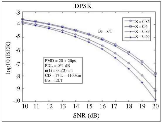
The electrical filter which we had used was the fifth order Bessel type, as we had done with the optical filter; we did with the electrical filter to get a best output. The best BER is found at Be T = 0.65. Also, here, PMD has a values of 20ps in each section, PDL has 0.5dB in each section, and CD=17 in each section. This is presented in figure (3).
Figure 2. Log (BER) versus SNR for several values of The optical filter (Be = 0.65/T ) PMD1 = PMD1 = 20 ps, PDL1 = 0, PDL2 = 1dB, CD1 = CD2 = 17
Figure 3. Log (BER) versus SNR for several values of The electrical filter (Be = 1.2/T ) PMD1 = PMD1 = 20 ps, PDL1 = 0, PDL2 = 1dB, CD1 = CD2 = 17)
References
[1] Caplan, D. O., Altia, W. A. (2001). A quantum-limited optically-matched communication link, In: Proc. Optical Fiber Commun. Conf. (OFC 01), Paper MM2.
PMD = 20 + 20ps PDL = 0*1 dB n(1) = 0 n(2) = 1 CD = 17 L = 1100km Bo = 1.2/T
X = 0.85 X = 0.6 X = 0.83 X = 0.65 DPSK
DPSK
-3
-4
-5
-6
-7
-8
-9
-10
log10 (BER)
Be = x/T
SNR (dB)
10 11 12 13 14 15 16 17 18 19 20 B0 = 2/T
B0 = 1.2/T B0 = 1/T
B0 = 1.6/T B0 = 1.8/T
B0 = 2.2/T
PMD = 20 + 20ps PDL = 0*1 dB n(1) = 0, n(2) = 1 CD = 17 Bo = 0.65
SNR (dB)
-2 -3
-4
-5
-6
-7
-8
-9
-10
log10 (BER)
[2] Henry, P. S. (1989). Error-rate performance of optical amplifiers, In: Proc. Optical Fiber Commun. Conf. (OFC 89), Paper THK3.
[3] Spisser, A., Ledantec, R., Seassal, C., Leclercq, J. L., Benyattou, T., Rondi, D., Blondeau, R., Guillot, G., Viktorovitch, P. Highy selective and widely tunable 1.55µm InP/air-gap micromachined Fabry-Perot filter for optical communications, Photon. Tech. Lett., 19 (9) 1259-1261.
[4] Irmer, S., Daleiden, J., Rangelov, V., Prott, C., Romer, F., Strassner, M., Tarraf, A., Hillmer, H. (2003). Ultralow biased widely continuously tunable fabry-Perot filter, Photon. Tech. Lett., 15 (3) 434-436.
[5] Chinn, S. R. (1995). Errr-rate performance of optical amplifiers with Fabrot filters, Elec. Lett., 31 (9) 756-757.
[6] Jacobs, I. (1990). Effect of optical amplifier bandwidth on receiver sensitivity, IEEE Trans. Commun., 38, p. 1863-1864.
[7] Olsson, N. A. (1989). Lightwave systems with optical amplifiers, J. Lightwave Technol., 7, p. 1071-1082.
[8] Forestiri, E. (2000). Evaluating the Error Probability in Lightwave Systems with Chromatic Dispersion, Arbitrary Pulse Shape and Pre-and Postdetection Filtering, J. Lightwave Technology, 18 (11) 1493-1503.
[9] Lima, I. T., Lima, A. O., Sun, Y., Jiao, H., Zweck, J., Menyuk, C. R., Carter, G. M. (2005). A receiver Model for Optical Fiber Communication Systems With Arbitrarily Polarized Noise, Journal of Lightwave Technology, 23, p. 1478-1490.
[10] Zhang, Z., Chen, L., Bao, X. (2007). Accurate BER Evaluation for Lumped DPSK and OOK Systems with PMD and PDL, Optics Express, 15 (15) 9418-9433, July.
[11] Golomb, S. W. (1967). Shift Register Sequences, San Francisco, CA: Holden-Day.
[12] Chen, L., Zhang, Z., Bao, X. (2007). Combined PMD-PDL Effects on BERs in Aimplified Optical Systems: an Analytical Approach, Opt. Express, 15, p. 2106-2119.