U
niversity of
T
rento
Department of Physics
Thesis submitted to the
DoctoralSchool inPhysics– XXXcycle by
E
leonora
F
ava
for the degree of
D
octor of
P
hilosophy
– D
ottore di
R
icerca
Static and dynamics properties of a
miscible two-component
Bose–Einstein Condensate
Supervisor: GabrieleFerrari
Co-Supervisor: Giacomo Lamporesi
Eleonora Fava
Static and dynamics properties of a miscible
two-component Bose–Einstein Condensate
Ph.D. Thesys in Physics
C O N T E N T S
introduction 1 1 theory 5
1.1 Weakly interacting trapped BECs at zero temperature 5 1.2 Quantum mixture at zero temperature 7
1.2.1 The buoyancy phenomenon 10 1.2.2 Collective oscillations 13 1.2.3 Static polarizability 13
1.2.4 Out-of-equilibrium mixture 14 1.3 Sodium properties 15
1.4 Weakly interacting trapped BEC at finite temperature 17 1.5 Quantum mixture at finite temperature 18
2 experimental apparatus 23
2.1 Atomic source and vacuum apparatus 23 2.2 Laser system 26
2.3 Magnetic fields 29 2.4 Optical-dipole trap 33
2.5 Electronic and control system 37 2.6 Imaging system 38
3 experimental methods 43 3.1 From laser cooling to BEC 43 3.2 Optical trap loading 46 3.3 Mixture creation 47
3.3.1 Landau–Zener transfer 48 3.3.2 Rabi coupling 50
3.3.3 µ-wave dressing 53
3.4 Calibration of the magnetic field~B 54 3.4.1 By 55
3.4.2 Bx 56 3.4.3 Bz 56
3.5 Heating procedure 57 3.6 Stern–Gerlach imaging 59 4 experimental results 63
4.1 Two-component BEC at T∼0 63 4.1.1 Trap frequencies 64
4.1.2 Calibration of the gradient 65
4.1.3 Measurement of the static polarizability atT∼0 67 4.1.4 Measurement of the spin dipole oscillation atT∼0 72 4.2 Two-component BEC at finite temperature 75
4.2.1 Collisional regimes 75
4.2.2 Traps frequencies and depths 77
4.2.3 Measurement of the spin dipole oscillation at finite
temperature 84
4.2.4 Measurement of the static polarizabiliy at finite
tem-perature 87
5.2 Passive magnetic shielding 94
5.2.1 Magnetic shield shapes performances 96 5.2.2 Materials 98
5.2.3 Degaussing 99 5.3 Shield constraints 100
5.4 Finite element method simulations 103
5.4.1 Introduction to finite element method (FEM) 103 5.4.2 Number of layers 103
5.4.3 Saturation 104
5.4.4 Inter-layer distance 107 5.4.5 Collar 110
5.4.6 Final design 111 6 conclusion 117
a appendix a 119
“Si sta come di primavera sul banco ottico gli AOM”
I N T R O D U C T I O N
Since the first realization of Bose–Einstein condensation [1, 2], the
ultra-cold gases established as a powerful platform of research both theoretically and experimentally. One of the main reasons which makes BECs a successful topic of research is their flexibility for creating systems whose Hamiltonian can be engineered almost at will. Thus, by preparing the proper experiment, it is possible to simulate and investigate a large variety of many-body config-urations related to several research fields in physics, from condensed matter to high-energy physics to cosmology. [3]. For instance, BECs can be used to
simulate spin-orbit coupling (SOC) in solid state matter physics [4], vorticity
in quantum and classic fluid-dynamics [5], Hawking’s radiation [6], the
uni-verse expansion [7], Mott-insulators [8] or high-Tc superconductivity [9].
In my thesis work, I will mainly focus on the study of spin properties in bi-nary Bose-Bose mixtures trapped in harmonic optical potentials. This topic is intrinsically related to spintronic, which is a rising field of research focused on the influence of electron (and nuclear) spin on the electrical conduction. Spin properties can be exploited in alternative or in addition to charge and orbital degrees of freedom. Spin relaxation and spin transport in metals and semiconductors are of high interest not only for their fundamental implica-tions, but also for their possible application in (spin)electronic technology. Nowadays, some devices based on the use of spin properties are already employed in industry, like giant-magnetoresistive (GMR) layers structures [10]. These devices are used as memory-storage cells or read head and
con-sist of alternate layers of ferromagnetic and non-magnetic metals, which are able to change their resistance depending on the magnetization on the mag-netic layers. However, they represent only a first step in the development of spintronics, since our understanding of many-body spin dynamics is still incomplete. In fact, the study of spin transport in solid-state physics is com-plex since in these systems spin is not a conserved quantity and different relaxation mechanisms can occur.
In this framework, the investigation of systems where spin is a conserved quantity can represent a starting point to deepen in the field. For example, degenerate binary mixtures can be investigated to study the role of interac-tions between different spin particles that, at finite temperature, can lead to a relaxation of the spin current via spin drag [11], as well as the condition to
spin superfluidity [12].
Another relevant field of research, which is very popular nowadays, con-cerns new phases of matter. Among all the fascinating new kinds of systems which have been predicted in the last decades, supersolids are particularly relevant in the field of Bose–Einstein condensation. This new phase of matter, was predicted for the first time by Thouless and independently by Andreev and Lifshitz in 1969 [13, 14]. A supersolid consists in a material where the
properties of superfluidity (intended as off-diagonal long-range order) and solidity (intended as density long-range order) can simultaneously exist [15].
The link between supersolidity and BEC lies on the possibility to engineer a quantum system, for instance by means of the spin-orbit coupling, in which diagonal and off-diagonal long range order coexist in the so-called stripe phase [16] and the experimental observation of the supersolid phase [17,18]
will permit to address several fundamental questions.
Technically, the realization of SOC-BEC in the stripe phase requires the ma-nipulation of degenerate binary mixtures under precise control of environ-mental magnetic fields in conditions that are difficult to meet in most ex-perimental apparatus. More specifically, the need to manipulate quantum binary mixtures requires a deep knowledge of the system properties, even in absence of coherent coupling (Ω = 0) between the two states, while to control the magnetic field with high precision, shielding tools are required. Both these topics are related to my research work, which aims to lay the foun-dation for experimental studies in resonantly-coupled spinor BECs, such as spin-orbit coupled BECs.
At this initial stage, the simplest collective oscillation,i.e., the spin-dipole (SD) oscillation and the static SD polarizability are studied to test the misci-bility properties of the system and its response to external perturbation of the trapping potentials, both in the static and in the dynamic case in order to characterize the response of the system at Ω = 0. In addition to its link with the realization of more complex binary systems, my research reveals interesting features concerning the spin properties of the |F = 1,mF = ±1i
binary mixture of sodium atoms. In fact, since this system is miscible and fully spin symmetric, it is possible to investigate its spin properties when a small displacement of the trap minima is applied,i.e., it is possible to inves-tigate the linear regime, where interactions among atoms play a crucial role. Differently from other mixtures already investigated [19, 20, 21, 22, 23, 24, 25,26,27,28,29,30,31, 32,33,34,35,36,37], the spin-dipole oscillation
fre-quencyωSD and the static SD polarizabilityP are directly studied. While the
SD oscillation shows interesting relations with the giant dipole resonance of nuclear physics [38], the investigation of this system at finite temperature
permitted to prove the superfluid nature of spin currents in the case of a collisional regime. In fact, the observation of undamped oscillations at zero temperature is consistent with superfluidity, but is not a proof of it, since undamped oscillations can be the result of mean-field interactions (as the propagation of spin-zero-sound in a normal Fermi liquid [39]). The
observa-tion of undamped spin oscillaobserva-tions in the collisional regime can be instead regarded as a direct proof of spin superfluidity since, in the presence of col-lisions, the spin current of the normal component is not conserved due to spin drag and only in the superfluid phase one can observe the propagation of spin sound.
contents 3
Thanks to the implementation of magnetic shielding and the use of a new experimental sequence to reach quantum degeneracy, it will be possible to study mixtures in the presence of a coherent coupling between the two states on timescale long compared to those of the many-body dynamics (Fis¯h project). Such systems show properties having analogies with the formation of stripe phases or with the formation of domain walls (as proposed by [40]),
which are related to quark confinement in quantum chromodynamics (QCD) .
In conclusion, my work represents only the starting point of a wider re-search that will be developed in the next years and that will lead to a deeper understanding of several systems and phenomena related to superfluidity and spinor physics.
The thesis is divided into five chapters, each of them dedicated to a specific topic.
• The first chapter is devoted to the theoretical description of harmoni-cally trapped binary mixtures of Bose-Einstein condensates both at zero and finite temperature. In particular, the conditions to have a miscible mixture are described, as well as the buoyancy phenomenon, which affects most of the binary mixtures studied so far. In this chapter the theoretical estimates of the spin-dipole oscillation frequency ωSD and
polarizability P, in the limit of linear regime, are given and the con-ditions at which these quantities can be experimentally measured are discussed.
• In the second chapter the experimental apparatus used to perform the experiment is described in detail, ranging from the vacuum apparatus to the experimental control system.
• In the third chapter all the experimental techniques used to create the binary mixture are presented. Here, particular attention is given to the sequence that allows to create and study the condensed binary system, both in the limit of low and finite temperature.
• In the fourth chapter I report on the main results concerning the static and dynamic spin properties of our binary mixture of BECs, which are studied both at zero and finite temperature. In particular, in the finite temperature case, two interacting regimes are investigated, namely col-lisionless and collisional. For both temperature conditions, a direct com-parison of experimental data with numerical integrated Gross–Pitaevskii equation (GPE) simulations is shown.
1
T H E O R Y
Contents
1.1 Weakly interacting trapped BECs at zero temperature 5 1.2 Quantum mixture at zero temperature 7
1.2.1 The buoyancy phenomenon 10 1.2.2 Collective oscillations 13 1.2.3 Static polarizability 13
1.2.4 Out-of-equilibrium mixture 14 1.3 Sodium properties 15
1.4 Weakly interacting trapped BEC at finite temperature 17 1.5 Quantum mixture at finite temperature 18
This chapter is devoted to the theoretical description of quantum-degenerate binary mixtures both at zero and at finite temperature. After a brief re-minder on the case of a weakly interacting BEC in a harmonic trap, the cou-pled Gross–Pitaevskii equations used to describe binary ultracold mixtures at zero temperature are derived. This theoretical approach, which holds at T =0, is then extended to the case of finite temperature using a mean-field description based on the Hartree–Fock approximation.
In addition, the miscibility conditions for a binary BEC mixture are also in-troduced, showing that the sodium system used for this work is an excellent candidate to study static and dynamic properties in the linear regime that were never previously studied.
1.1
weakly interacting trapped becs at zero
tem-perature
The theoretical description of our system should take both interactions and the confining potential into account. Even if the mean-field theory de-veloped by Bogoliubov in1947[41] is able to describe the role of interactions
among particles, it is not suitable to describe the role of external potentials. Since most experiments with ultracold atoms are performed in traps (mag-netic or optical), it is important to properly describe these non-uniform sys-tems.
The generalization of the Bogoliubov theory to the case of non-uniform and time-dependent configurations can be obtained assuming that, to the low-est approximation, the field operator ˆΨcan be replaced by the classical field
Ψ(~r,t), called the order parameter [42]. This approximation holds at very low
temperature and for a large number of particles. In addition, since for dilute
cold gases only binary collisions are relevant at low energy, the interaction among particles can be described by a contact potential
V(~r0−~r) = gδ(~r0−~r), (1.1)
where the coupling constant g is directly related to the s-wave scattering length atrough the relation
g= 4πh¯
2a
m , (1.2)
¯
his the Planck constant andmis the particles mass. These assumptions lead to the Gross–Pitaevskii equation (GPE) [42]
i¯h∂
∂tΨ
(~r,t) = −¯h 2∇2
2m +Vext(~r) +g|Ψ(~r,t)| 2
!
Ψ(~r,t), (1.3)
whereVextis the external potential used to trap the sample.
For a gas confined in a harmonic trap, the external potential at a given position~r, can be expressed as
Vext(~r) =Vext(x,y,z) =
1 2mω
2 xx2+
1 2mω
2 yy2+
1 2mω
2
zz2, (1.4)
whereωx,y,z are the trapping frequencies. The size of the atomic cloud along
each direction iis fixed by the harmonic oscillator length
ahoi =
p
¯
h/mωi. (1.5)
The characteristic length of the system is thus given byaho= √h¯/mω¯, where ¯
ω= (ωxωyωz)1/3 is the geometrical average of the trapping frequencies. The
ground state of Eq.1.3 is obtained, within the formalism of mean field, by
writing the wave function asΨ(~r,t) =φ(~r)e−iµt/¯h
µφ(~r) = −¯h 2∇2
2m +Vext(~r) +gφ 2(~r)
!
φ(~r) (1.6)
When the energy contribution due to interactions is large compared to the
Thomas–Fermi limit
kinetic energy of the system, the so-called Thomas–Fermi approximation is applicable. In this limit the kinetic energy (also called the quantum-pressure) is neglected and the Gross–Pitaevskii equation (Eq.1.6) reduces to
µφ(~r) = Vext(~r) +gφ2(~r)φ(~r), (1.7)
from which the density profile of the trapped BEC can be extracted
n(~r) =φ2(~r) = µ−Vext(~r)
g . (1.8)
From Eq.1.8 some of the quantities used in the next chapters are obtained,
such as the chemical potential and the Thomas–Fermi radii which are
µ= h¯ω¯
2
15Na aho
2/5
1.2 quantum mixture at zero temperature 7
and
Ri = s
2µ
mωi, (
1.10)
respectively. Other important quantities which will be used later in the thesis, are the healing length ξ and the critical temperature TC. The former can
be interpreted as the recovery length of the condensate, i.e., the distance necessary to restore the local equilibrium value of the densitynfrom 0 and is defined as
ξ = r
1
8πna. (
1.11)
The critical temperatureTCcorresponds to the temperature below which the
condensation occurs. Since interactions in the estimate of TC generally give
a small correction, the critical temperature is computed using the formula valid for trapped non-interacting systems
TC =
¯ hω¯
kB
N
ζ(3) 1/3
, (1.12)
wherekB is the Boltzmann constant andζ is the Riemann zeta function.
1.2
quantum mixture at zero temperature
The advent of optical traps for quantum gases [43] has opened an
inter-esting scientific scenario, both experimentally and theoretically. In fact, the possibility to trap atom independently from their internal state paved the way for the realization of more complex systems that can be engineered with great flexibility. In the last twenty years, several spinor systems, i.e., systems in which atoms occupy each level of the given hyperfine manifold, were realized using both rubidium [44, 45, 46] and sodium [47, 48, 49, 50]
atoms in the F = 1 ground state. In addition, several theoretical works and reviews are reported in literature [51,52,53,54, 55], also concerning spin-2
systems [56,57].
Of particular interest for this thesis work are binary mixtures, which are widely investigated due to the large variety of systems that can be created [58,59,60,61,62,63,64,65,66]. In fact, it is possible to obtain experimentally
binary mixture using different atomic species ( like K-Rb[23,24], Yb-Li [36],
Yb-Cs [35], Rb-Cs [30] or Na-K [28]) or using two isotopes of the same atom
(like 6Li-7Li in [67, 29, 31] or 4He-6He in [68]). Another class of mixtures
which attracts large interest corresponds to mixtures obtained using two in-ternal states of the same atomic species. These states can be two Zeeman levels of the same hyperfine level ( like in rubidium [21,22,32], in sodium
[69, 33] or in potassium [37]) or can belong to two hyperfine states (like for
the case of87Rb in [19,20,25,26,27,34]).
|2, 1i+|1,−1iof rubidium [25, 20, 34]. This mixture, being at the
miscible-immiscible threshold (see Subs.1.2.1), presents a non-trivial dynamics which
can lead to the formation of ring excitations (in absence of Rabi coupling between the two spin components).
Other works related to my research, concern the study of dynamics on both sides of the miscible-immiscible phase transition by means of Feshback res-onance in |2,−1i+|1, 1imixture of rubidium atoms.
However, all these works focus on dynamics properties of system which are not fully miscible (see next subsections), while, in my research, dynamic and static spin properties [70] of a completely miscible mixture are investigated.
In the following a theoretical description of binary mixture is reported, giv-ing particular attention to the concept of miscibility.
In the case of a single component BEC, interactions are well described
Binary interacting mixtures
by a single parameter, i.e., the coupling constant g. In a binary mixture, it is necessary to introduce three parameters to describe all the interactions occurring in the system. Labeling the two condensates as 1 and 2, these pa-rameters are g11, g22 and g12 which are the two intra-component coupling
constants and the inter-component coupling constant, respectively.
The first theoretical description of a binary mixture was presented in 1996
[71] and it is obtained generalizing the GP equation for the two condensates,
where each component is described by its own wave function. Proceeding in this way the energy of the mixture can be written as
E= Z
d~r
"
¯ h2 2m1
|∇Ψ1|2+ ¯h
2
2m2
|∇Ψ2|2+V1,ext|Ψ1|2+V2,ext|Ψ2|2
+1
2g11|Ψ1|
4+1
2g22|Ψ2|
4+g
12|Ψ1|2|Ψ2|2,
(1.13)
whereΨ1,Ψ2are the wave functions of the condensates,m1,m2their relative
masses andV1,ext,V2,extare the trapping potentials experienced by each
com-ponent. The coupling constantsg11 =4π¯h2a11/m1andg22 =4πh¯2a22/m2are
fixed by the s-wave scattering lengths a11,a22 which characterize the
interac-tion between pairs of atoms of the same condensate, whileg12=2π¯h2a12/mr
counts for interactions between atoms of different species, being 1/mr =
1/m1+1/m2the reduced mass. In order to guarantee the stability of the
sys-tem, g11 andg22 are assumed to be positive, whileg12 can be either positive
or negative [42].
From the variational principle it is possible to obtain the coupled Gross– Pitaevskii equations which describe the two components of the system
i¯h∂
∂tΨ1= −
¯ h2∇2
2m1
+V1,ext(~r) +g11|Ψ1|2+g12|Ψ2|2 !
Ψ1 (1.14)
i¯h∂
∂tΨ2
= −h¯ 2∇2
2m2
+V2,ext(~r) +g22|Ψ2|2+g12|Ψ1|2 !
Ψ2 (1.15)
and from which the ground state of the mixture can be found.
For simplicity we start by considering the equilibrium regime in a
homo-Uniform system
1.2 quantum mixture at zero temperature 9
or in a phase separated configuration. In the uniform case the interaction energy takes the form
Euni f =
g11 2 N2 1 V + g22 2 N22
V +g12 N1N2
V , (1.16)
while in the separated configuration it takes the form
Esep=
g11
2 N12 V1
+ g22 2
N22 V2
, (1.17)
whereV1andV2are the volumes occupied by the two separated components
andV= V1+V2is the total volume.
The mechanical equilibrium between the two separated phases is given by the condition
∂Esep ∂V1
= ∂Esep
∂V2
, (1.18)
which implies the relationship
g11
N1 V1
2
= g22
N2 V2
2
. (1.19)
By substituting Eq.1.19 in Eq.1.17, one finds
Esep=
g11
2 N12
V +
g22
2 N22
V +
√
g11g22 N1N2
V . (1.20)
The condition to avoid phase separation is Esep > Euni f which, comparing
Eq.1.20 and Eq.1.16, leads to the relation g12 < √g11g22. This condition can
be generalized, in the case of attractive interactions between the two spin components, by considering that the uniform phase is stable against ener-getic instabilities1
if
|g12|< √
g11g22. (1.21)
When this condition is satisfied the system is said to be miscible, while when the system is in the phase separated configuration, it is said to be immiscible. In Fig.1.1an example of both miscible and immiscible systems are reported
for the case of atomic sodium.. The miscible system correspond to the mix-ture |F = 1,mF = ±1i (right image of Fig.1.1), while the immiscibility is
visible in the spinor configuration, where all three levels of sodium ground state F = 1 are present (left image of Fig.1.1). In the spinor, the phase
sep-aration is due to the presence of|F = 1,mF = 0i, which is immiscible with
both|F=1,mF=1iand|F=1,mF= −1i. Trapped system
In the trapped configuration the equilibrium density profiles can be ob-tained in the Thomas–Fermi limit (described in Sec.1.1) where, under the
miscibility condition, one finds that Eqs.1.14,1.15become
µ1−V1,ext(~r)−g11n1(~r)−g12n2(~r) =0 (1.22) µ2−V2,ext(~r)−g22n2(~r)−g12n1(~r) =0. (1.23)
1 Actually, if|g12|>√g11g22, quantum fluctuations prevents the collapse of the system,
Figure 1.1: Comparison between a phase separated spinor (left) and miscible
mix-ture(right). The phase separated system is composed of the three Zeeman sub-levels of the ground state of sodium, while the miscible system is composed of the two zeeman sublevels |F = 1,mF = 1i and |F = 1,mF = −1i. The phase
separation in the spinor configuration is due to the presence of|F =1,mF = 0i,
which is immiscible either with |F = 1,mF = 1i and |F = 1,mF = −1i. Both
the pictures were taken after TOF in a Stern–Gerlach configuration in order to spatially separate the different spin components.
These equations hold, provided n1(~r)andn2(~r)are finite or set to zero and,
in the region of non-vanishing densities, they can be rewritten as
n1(~r) =
1 g11(1−∆)
µ1−
g12 g11
µ2−V1,e f f(~r)
(1.24)
n2(~r) =
1 g22(1−∆)
µ2−
g12 g22
µ1−V2,e f f(~r)
(1.25)
where∆= g212/g11g22 <1 and
V1,e f f(~r) =V1,ext(~r)−
g12 g22
V2,ext(~r) (1.26)
V2,e f f(~r) =V2,ext(~r)−
g12 g11
V1,ext(~r) (1.27)
are the effective potentials felt by the two components.
A relevant feature emerging from the equations reported above is that the Thomas–Fermi radii of the two components are in general not equal. This feature is related to an interesting phenomenon known as buoyancy which is the topic of the next section. It is important to note that, when dealing with quantum mixtures, the TF approximation can be considered valid when the TF radii are much larger than the spin healing length
ξs=h¯/ q
2mn(√g11g22−g12). (1.28)
1.2.1 The buoyancy phenomenon
1.2 quantum mixture at zero temperature 11
one where the two components tend to stay apart one from the other, oc-cupying different volumes, depending on the interaction properties of the system.
As matter of fact, even when the system is in the miscible configuration, the density distributions of the two components can rearrange themselves in a non-obvious way. This phenomenon is related to the intra-component cou-pling constants and appears only wheng11 andg22are not equal and when
atoms are confined in a non-uniform potential.
Let us suppose, for example, thatg22> g11andN1 =N2and let us consider
the peak density distributions of the single component in the Thomas–Fermi approximation
ni(0) = µi
gii
. (1.29)
Sinceµ∝g2/5 it is simple to verify that
n2(0) n1(0) ∝
g11 g22
3/5
<1, (1.30)
thus n2(0) < n1(0). This inequality underlines the fact that, even without
taking the inter-component interactions into account, the two components have different density distributions and Thomas–Fermi radii.
In addition, the interaction term between the two components propor-tional to g12n1n2 is not negligible and its effect is to increase the internal
energy of the system. Thus, to minimize the total energy, the energetic con-tribution given by the interaction between atoms of different components should be reduced.
In order to weaken this interaction energy the system has the only possibil-ity to change the two denspossibil-ity distributions in order to reduce the overlap area between the two components. Thus, using the same example as before, the denser component 1 will tend to shrink even more increasing its peak density and reducing its TF radius, while component 2 will tend to decrease its peak density. In addition, the inverted-parabola profile will be modified in order to further reduce the density in the overlap area and, consequently, increasenoutside the spatial region occupied by component 1. A sketch of this rearrangement mechanism is given in Fig.4.2. This phenomenon goes by
the name of buoyancy since the overall effect is that one component "floats" on the other, being the two density distributions related one to the other. The buoyancy issue is a fundamental one because, even if strictly speak-ing the system is miscible, the density distribution profiles are modified by interactions. This phenomenon can lead to a non-harmonic dynamics of the system and instabilities, which are generally difficult to describe. In addition, it prevents the direct measurements of spin properties like static spin-dipole polarizability P or spin-dipole oscillation frequencyωSD, which are visible
when the trap minima (hence density distributions) are slightly displaced one respect to the other from their common rest position (see next subsec-tions).
Figure 1.2: (a) Sketch of the density distribution arrangement in the case of a
mis-cible mixture whereg11 6= g22 and g12 = 0. The effect of having different
intra-coupling constants is to create two density distributions with different TF radii. (b) Comparison between the density distributions arrangement in the case of a miscible mixture withg11 6= g22 with (solid line) and without (dotted line)
inter-component interaction. Due to inter-inter-component interaction the system tends to reduce the overlap are of the two atomic cloud by shrinking the density distribu-tion of component 1 and by modified the inverted-parabola profile of component 2.
In a uniform binary mixture, the frequency of the Bogoliubov modes is
ωd,s = v u u t
¯ h2k2
2m ¯ h2k2
2m +2mcd,s
!
(1.31)
where, assuming that m1 = m2, n1 = n2 = n/2 and g11 = g22 = g, the
density (d) and spin (s) sound velocities are given by [42]
c2d,s= n
2m(g±g12). (1.32)
The + sign corresponds to density oscillation where the two fluids move in phase, while the − sign is associated to out-of-phase spin oscillation. An interesting question concerns the stability of the system when the two fluids can move at velocities v1 andv2 and the sound velocity, which corresponds
to the leading term in the Bogoliubov dispersion relation at small~k, is
cd,s= r
c20+ 1 4v
2±qc2
0v2+c40g122 /g2±V, (1.33)
where c2
0 = gn/2m, v = v1−v2, V = (v1+v2)/2 and v1,v2 and~k are
assumed to lie on the same axis. Here, the condition for having stability is more complex than the single component case, where the Landau criterion [42] holds. In fact, the term ±V provides the instability associated to the
Landau criterion if c becomes negative (energetic instability), whilev plays a role in the dynamic instability. If cs < |v|/2 < cd (where cd,s are given
by Eq.1.32), the solution of Eq.1.33 is imaginary and the system shows a
dynamic instability. Similarly, if v > cd, c is real but the system develops
1.2 quantum mixture at zero temperature 13
1.2.2 Collective oscillations
Generalizing the hydrodynamic formalism developed for a single BEC [74], it is possible to study collective oscillations of mixtures of BECs trapped
in harmonic potentials. In particular, in the simplest symmetric case ofN1 = N2 and g11 = g22 = g, the equation of the density oscillation remains equal
to the case of a single component BEC
∂2
∂t2δn=∇ ·
c2(~r)∇δn
(1.34)
where δn(~r,t)=n−n(~r) is the change of the density profile with respect to
the equilibrium profile andmc2(~r) =gn(~r).
Instead, the equation for the spin density fluctuations for mixtures of BECs is different from the one describing the case of a single component BEC, reading as
m∂ 2
∂t2δs(~r) = (g−g12)∇ ·[n(~r)∇δs(~r)] ( 1.35)
whereδs(~r) =δn1(~r)−δn2(~r)[42].
Since the equilibrium density profile is not modified and keeps the form n(~r)=(µ−Vext(~r))/g, all discretized collective frequencies holding for a
sin-gle component BEC are still valid for a symmetric mixture simply introduc-ing a normalization factorp(g−g12)/g.
Of particular interest is the spin-dipole (SD) oscillation, in which the two- Spin-dipole oscillation
spin clouds move one with respect to the other with opposite phase. In the case of small oscillation amplitude with respect to the size of the condensates (linear regime), the relative motion is essentially "internal" since the edges of the density distributions do not move (as seen from GPE simulations). For the case of symmetric mixtures, the frequency of the spin-dipole oscilla-tion [42,70] can be expressed as
ωSD = s
g−g12 g+g12
ωho. (1.36)
The spin-dipole oscillation frequency is the simplest collective oscillation which is supported by the system and it can give information on the spin dynamics, as well as on the thermodynamics of the system. This frequency is predicted to be sensitive to the vicinity of the miscible-immiscible phase transition [70,60].
So far, a direct measurement of this frequency was missing since the phe-nomena of phase-separation or buoyancy between the two spin components prevent observing this oscillation in the linear regime. Nevertheless, we mea-sured it in Trento using a completely miscible mixture of sodium atoms (see Sec.1.3and Ch.4).
1.2.3 Static polarizability
the ability of the system to adapt to a relative displacement of the trapping potential minima for the two components and it is defined as
P = x1−x2 2x0
(1.37)
wherex1−x2 is the distance between the centers of mass of the density
dis-tributions of the two spin components and 2x0is the total distance between
trap minima. This quantity exhibits a divergent behavior at the transition between the miscible and immiscible phases where important spin fluctua-tions can occur [61,64].
The static SD polarizability is directly linked to the SD oscillation
pre-Relation betweenωSDand
P sented in the previous section. This relation emerges when the SD
oscilla-tion frequency is computed using the sum rule approach, which applies for small displacements of the trap minima with respect to the sample size. In this framework, it is possible to introduce the energy weighted m1(SD)and
the inverse energy weighted moment m−1(SD)of the spin-dipole dynamic
structure factorSSD(ω)which reads as
SSD(ω) =Q−1
∑
m,ne−En/kBT|hn|S
D|mi|2δ(¯hω−h¯ωnm) (1.38)
whereSD = ∑kxkσzk is the spin dipole operator, ωnm = (En−Em)/¯hare the
Bohr frequencies and Q= ∑me−Em/kBT is the partition function. The energy weighted moment [42] is model independent and it is given by
m1(SD) =N¯h2/2m. (1.39)
The inverse energy weighted moment is given by
m−1(SD) =
NP
2mω2x, (
1.40)
whereP is fixed by the ratio between the induced spin displacement of the atomic clouds and the separation 2x0 of the two harmonic traps [70].
The estimate ofωSD is provided by the ratio
¯ hωSD=
s
m1(SD)
m−1(SD)
, (1.41)
hence, using Eqs.1.41, 1.39 and 1.40, the linear SD polarizability P can be
computed atT =0 from the value ofωSD using the relation
ωSD = ωx √
P. (
1.42)
1.2.4 Out-of-equilibrium mixture
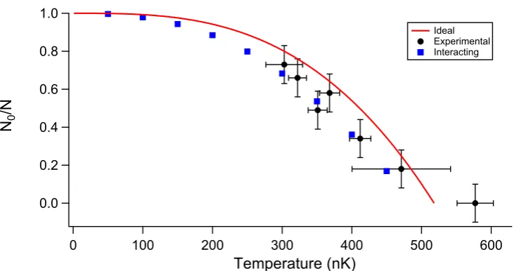
1.3 sodium properties 15
Let us consider a polarized sample at finite temperatureTwith a total num-ber of atomsN. Typically, a fraction of the atoms is condensed (N0/N), while
the remaining (NT/N) belong to the thermal cloud, such that
N= N0+NT. (1.43)
The splitting of the sample into two systems having N/2 atoms each, con-serves the total number of particlesNbut not the temperatureT. In fact, one can describe the system before the splitting and after in the new equilibrium configuration (labeled as ’) as
N= N0+NT
N=2N00 +2NT0.
The number of condensed atoms (N00) and the number of thermal atoms (NT0) in each sample after the splitting, can be estimated by considering that the main energetic contribution is given by the internal energy of the thermal distribution in the trapping potential, which is equal to
U =3NTkBT. (1.44)
Considering that for an ideal Bose gas in harmonic confinement NT ≡
N−N0 = ξ(3)
kBT
¯ hω¯
3
, where ξ(n)is the Riemann ξ function and
impos-ing energy conservation across the splittimpos-ing procedure, one finds that the temperature of the systems reduces since
T0 ∼0.85T (1.45)
From the new value of the temperature T0 one can also estimate the new value ofNT0 andN00, which are
NT0 =0.6NT and N00 = N0
2 −
NT
10. (1.46)
This proves that, even if the absolute temperature of the system is lower, the two BEC distributions have less than half the initial number of condensed atoms. In fact some of the condensed atoms will be converted into thermal particles in order to conserve the energy of the system.
1.3
sodium properties
In the previous section I have described systems made of two components, showing that binary mixtures can be either miscible or immiscible. While in the immiscible regime the two components tend to stay apart from one other, in the miscible one they tend to occupy the same volume. In practice, this is not always true. Because of buoyancy, in fact, the two condensates tend to rearrange their density distributions, preventing the possibility to study the dynamics of the system in the linear regime.
atoms of the same atomic species occupying two different internal states. So far, most works were realized using rubidium atoms [19,20,75,26,27,32].
Even if rubidium presents the great advantage of having accessible Feshbach resonances [76] for several mixture combination, the mixtures created to date
present miscibility constrains since they can be either immiscible or affected by buoyancy.
An example of mixture extremely close to the phase transition and affected by buoyancy is reported in Fig.1.3, which corresponds to the case of a |F =
1,mF =−1iand|F=2,mF =1iRb mixture.
Figure 1.3: Experimental density profiles of the |2, 1i+|1,−1irubidium mixture
taken from [20]. The|1icomponent corresponds to the|2, 1istate, while|2i
cor-responds to the|1,−1istate. The density profile of|1i(a) is larger and presents a crater in the region occupied by the|2iatoms (b). (c) Density distribution of|1i
after introducing a non-zero relative sag.
From Fig.1.3one can observe that component|1ihas a larger distribution
with respect to component |2i, sinceg11 > g22. In addition, it is visible that
component|2itends to minimize its volume, while the density distribution of|1ishows a depletion where the two components overlap. Thus, it is clear that these systems are not suitable to study static and dynamic properties in the linear regime, being not miscible in a strict sense.
In this scenario, the sodium mixture |F = 1,mF = ±1iis the ideal plat-Completely miscible sodium
mixture form to study both static and dynamic properties in the linear regime, since
it is completely miscible and symmetric [77]. In fact, it does satisfy the
mis-cibility condition |g12|< √
g11g22,N1 =N2and, since at low magnetic fields g11 =g22= g, it is also not subject to buoyancy.
The values of the s-wave scattering lengths for the ground states of sodium (taken from [78]) are
a11 =a22=54.54(20)a0 and a12 =50.78(40)a0 (1.47)
wherea0is the Bohr radius.
Since g12 ∼ g the system is close to the miscible-immiscible phase
1.4 weakly interacting trapped bec at finite temperature 17
for the enhancement of the static SD polarizability with respect to the non-interacting system. Also the value of the SD oscillation frequency is sensitive to interactions, being five time smaller than the trap frequency.
Thus, the vicinity to the miscible-immiscibile phase transition is important since it permits to observe sizable interaction effects. However, when the system is extremely close to the phase transition (like in [20]) it is
diffi-cult to precisely control and study the system since it is deeply sensitive to other effects, such as asymmetries in the trapping potential [79]. In our
case, (g−g12)/g ' 7% and the system can be consider stable, even if it is
close enough to the miscible-immiscible transition to ensure sizable interac-tion effects.
1.4
weakly interacting trapped bec at finite
tem-perature
AtT 6=0, the condensate density is modified because of thermal depletion and interactions with the thermal component should be taken into account.
The simplest theory describing the thermodynamic behavior of a trapped Hartree–Fock approximation
interacting Bose gas at finite temperature is based on the Hartree–Fock (HF) approximation [80,81]. This theory assumes that, at equilibrium, the system
can be described as a gas of statistically independent single-particle excita-tions, whose average occupation number of theistates is ni =haˆiaˆii, being
ˆ
a and ˆa the single-particle creation and annihilation operator.
The energy of the system can be calculated by keeping only terms with an even number of creation/annihilation operators and setting
haˆiaˆki=niδik (1.48)
haˆiaˆjaˆkaˆli=ninj(δikδjl+δilδjk) (1.49)
The thermal and condensed components can be separated by associating the role of the thermal part to the excited states i 6= 0 and the role of BEC to the lowest energyi =0 state. Proceeding in this way the total energy of the system can be written as
E= Z
d~r[¯h
2
2mN0|∇ϕ0| 2+
∑
i6=0
¯ h2
2mni|∇ϕi| 2+V
ext(~r)(n0(~r) +nT(~r))
+g 2n
2
0(~r) +2gn0(~r)nT(~r) +gn2T(~r)]
(1.50)
where the density of the condensate and thermal parts are
n0(~r) =N0|ϕ0(~r)|2=|Ψ0|2 and nT(~r) =
∑
i6=0ni|ϕi(~r)|2,
respectively andϕi(~r)are single particle wave functions normalized to unity.
The average occupation number ni can be found by minimizing the energy
at fixed entropy andN, yielding to the Schrödinger-like equation
δE
δϕ∗i
where ei is the energy of the isingle-particle level. From Eq.1.51, when the
chemical potential approaches the energye0, one finds
−h¯ 2∇2
2m +Vext(~r) +g[n0(~r) +2nT(~r)]
!
Ψ0=µΨ0 (1.52)
for the BEC part and
−h¯ 2∇2
2m +Vext(~r) +2gn(~r)
!
ϕi(~r) =eiϕi(~r) (1.53)
for the excited single-particle states, where n(~r) is the total density of the system.
With respect to the GPE1.6, Eq.1.52 takes into account the interaction with
the thermal component being given by 2gnT, where the factor2comes from
the exchange term in the calculation ofE.
1.5
quantum mixture at finite temperature
The HF theory presented in the previous section is able to describe the thermodynamic behavior of the single component system in the presence of a thermal fraction. As seen in Sec.1.2, when dealing with a multi-component
systems, the role of inter-species interaction should be taken into account as well. To do so, one has to replace the coupling constant g of the single component system, with the three coupling constantsg11,g22andg12
charac-terizing interactions in a binary mixture.
In this framework Eq.1.52can be rewritten, for each of the two component,
as
µΨ1 = "
−h¯ 2
2m∇ 2+V
1+g11(n01+2n1T) +g12(n02+nT2) #
Ψ1 (1.54)
µΨ2 = "
−h¯ 2
2m∇ 2+V
2+g22(n02+2n2T) +g12(n01+nT1) #
Ψ2 (1.55)
whereg11,22 =4π¯h2a11,22/mandg12 =2πh¯2a12/m. The condensate densities
are given by n0
1,2 = |Ψ1,2|2 where we have assumed N1 = N2. The densities
of the thermal distributions are described by the semi-classical equation
nT1,2(~r) = 1 (2πh¯)3
Z
d~p f1,2(~p,~r,t), (1.56)
where the Wigner distribution function of the thermal atoms [82] is given by
f1,2(~p,~r,t) ={eβ[~p
2/2m+UT
1,2−µ1,2]−1}−1 (1.57)
and the effective potentials for the thermal fluids are
1.5 quantum mixture at finite temperature 19
Considering the Bose function
g3/2(z) =
2 √ π Z ∞ 0 dx √ x
z−1ex−1, (1.60)
Eq.(1.56) can be simplified to
nT1,2 = g3/2(z1,2)/λ3T (1.61)
whereλT = q
2π¯h2/(mkBT)is the de Broglie wavelength and
z1,2 = exp[(µ−U1,2T )/kBT] (1.62)
is the local fugacity of the spin components 1 and 2.
The equations reported above can be solved to find the ground state den- SD polarizability at finite T
sity distributions of the condensate and thermal atoms in the presence of the displacement 2x0between the harmonic traps, obtaining thus the
polarizabil-ity of the system as a function ofx0and temperature. In this framework, the
displaced potentials reads
V1=Vho(x−x0,y,z) and V2= Vho(x+x0,y,z) (1.63)
and, for the case of symmetric systems,µ1= µ2 =µ.
The BEC spin density, which corresponds to the relative distance between the two condensed component, can be found at low temperature by apply-ing the Thomas-Fermi approximation and neglectapply-ing the interaction between the condensate and the thermal component as well as thermal-thermal inter-actions in the Gross-Pitaevskii equations (1.54,1.55). This yields to
S0= n01−n02 =−x0
g+g12 g−g12
∂n0
∂x , (
1.64)
while for the thermal part one finds
STin =n1T−nT2 =− 1
kBTλ3Tz
∂g3/2(z)
∂z
2g g−g12
mω2xx0
in the inside region where the thermal part interacts with the condensate. In addition, without any external perturbations, one has
∂nT ∂x =
1 kBTλ3Tz
∂g3/2(z)
∂z
2g g+g12
mω2xx0,
so that
STin =n1T−nT2 =−x0
g+g12 g−g12
∂nT
∂x , (
1.65)
In a similar way the spin density of the outermost thermal component can be derived finding that
STout=nT1 −nT2 =−x0 ∂nT
∂x . (
The polarizability of the condensed (P0) and thermal (PT) part are found by
integrating their spin density
P0 = Z
xS0d~r/N0 (1.67)
and
PT = Z
xSTd~r/NT. (1.68)
From Eqs.1.64,1.65and1.66two main aspects emerge. One is the distinction
between the thermal atoms occupying the region where the BEC is present from the atoms occupying the region outside the BEC distribution. The sec-ond aspect regards the presence of the term (g+g12)/(g−g12)both in the
spin density of the condensed and thermal internal part. Both these argu-ments underline the importance of the inter-component interaction, which causes an enhancement of the polarizbility of the system.
1.5 quantum mixture at finite temperature 21
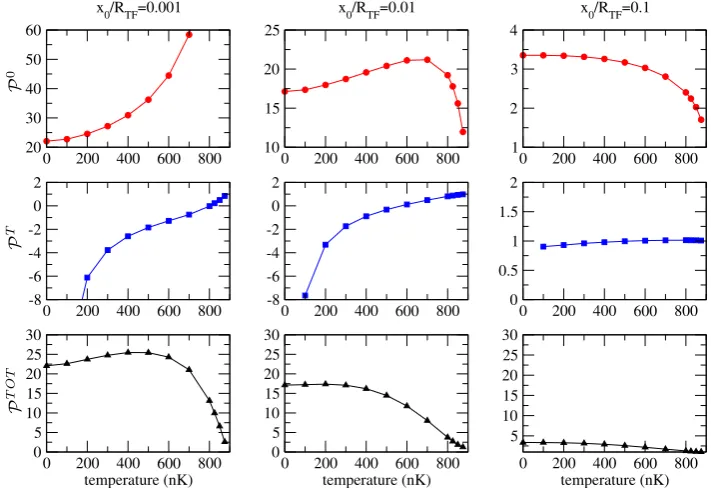
Figure 1.4:Computed SD polarizability of the condensedP0(upper row), thermal
PT(middle row) and totalPTOT(bottom row) atoms as a function of temperature
in the case ofN1= N2 = 105 and (ωx,ωy,ωz)=2π(44.5,1400,1400)Hz. In the left
column are reported the results obtained forx0/Rx=0.1%, in the central column
the results obtained for x0/Rx = 1% and in the right column are the results
obtained for x0/Rx = 10%. The critical temperature of the system computed
for a non-interacting system is930nK. The(g+g12)/(g−g12)which affects the
polarizability of both BEC and thermal cloud is relevant only in the linear regime
x0P RTF, which corresponds to the first column of the figure. Increasing the
displacement of the trap minima, interactions between spin components become less important leading to polarizability contributions close to 1 (third column).
In the same figure the behavior of the polarizability associated to the ther-mal cloud and the total polarizability, which is computed as
PTOT = N0P0+NTPT
N , (1.69)
are shown for different value ofx0.
From the simulations, it emerges that both the condensed and the thermal polarizability are modified by their mutual interaction, while the total polar-izability remains, in first approximation, equal to the one expected for the T=0 case.
Additional comments on the SD polarizability and its physical meaning are reported in Chapter4, where the main results of my research work are
2
E X P E R I M E N T A L A P P A R A T U S
Contents
2.1 Atomic source and vacuum apparatus 23 2.2 Laser system 26
2.3 Magnetic fields 29 2.4 Optical-dipole trap 33
2.5 Electronic and control system 37 2.6 Imaging system 38
Experiments with ultracold gases require well controlled experimental conditions where many physical parameters must be precisely varied in a reliable way. To fulfill these requirements a control over many instruments is typically needed. In this chapter I will present a detailed description of the experimental apparatus. First the atomic source and the vacuum apparatus are described. Then the laser systems used to produce visible and infrared radiation are described. The following section is devoted to the description of the magnetic trap used to create the BEC and, more in general, all the coils and their use is also illustrated. After the magnetic trap the dipole trap is presented in detail. The electronic control system is also described, making it clear how we control all the different steps of the experimental sequence. Finally the description of the imaging setup is reported in the last section, where the fitting procedures are also explained.
2.1
atomic source and vacuum apparatus
Atomic source
Since the first observations of the Bose–Einstein condensate with rubidium and sodium atoms [1,2], the interest in this kind of systems has considerably
grown, leading to the development of new efficient atomic sources. Atomic sources based on laser cooling can be divided into two main classes.
• A first class exploits dissipative light forces and inhomogeneous mag-netic fields to slow down a thermal flux of atoms which are coming from an oven. An usual implementation of this type of sources is the Zeeman slower (ZS), a stage where fast atoms are slowed down by means of a counter-propagating laser beam and a specific configura-tion of the magnetic field [83]. The slowed atoms can then be trapped
and cooled in magneto-optical traps (MOTs) [84].
• The second class of atomic sources uses atomic vapors directly loaded and cooled in a MOT: these setups present a simple design, but they provide satisfying performances only for medium and heavy atoms like potassium, rubidium and cesium [85,86,87].
Working with light alkali species (such as sodium or lithium) can lead, in case of a highly efficient Zeeman-Slower (ZS) stage, to experiments with a higher number of atoms [88] with respect to experiments performed with
heavier atoms. Anyway, even if these systems are suitable to capture a large number of atoms, they present some nontrivial drawbacks. Firstly, the ZS stage can be affected by losses due to the atomic beam divergence. Secondly the experimental apparatus is necessarily larger and more complex to oper-ate.
In2009a new type of atomic source based on a2D MOT stage was developed
for lithium [89], leading to more compact experiments without affecting the
total number of captured atoms.
The system used in our experiment [90] extended this approach to sodium
atoms, combining a2D MOT with a compact ZS stage.
Our atomic source is based on an oven filled with metallic sodium which is heated up to 250 ◦C (more than 150 ◦C above the melting temperature)
allowing atoms to evaporate in the vacuum system. The atomic cloud pro-duced by the evaporation is moving upward generating a flux that permits to transversely (y-zplane) load the2D MOT. In addition, using a laser beam
pointing opposite to the flux direction, it is possible to implement a ZS, which enhances the flux by more than an order of magnitude.
The magnetic fields required to operate the2D MOT and the ZS are obtained
by means of four sets of permanent magnets located close to the 2D-MOT
plane (see Fig.2.1).
Finally, a resonant-light beam aligned along the axial unconfined direction x, labeled as push beam, is used to push the atoms towards the final sci-ence chamber located∼30cm away from the2D MOT creating a collimated
atomic beam with a flux of more than4×109 atoms per second.
Beams and magnets positions are illustrated in Fig.2.1.
Figure 2.1: Scheme of the vacuum apparatus showing the position of the pumps,
the light beam directions and the location of the permanent magnets. On the right a magnified detail of the2D-MOT plane is reported.
Vacuum system
2.1 atomic source and vacuum apparatus 25
the ZS are located and the ultra-high-vacuum (UHV) chamber where a pres-sure lower than 1×10⁻¹⁰ mbar is reached and the experiment is carried out. These two parts are joined together via a differential pumping channel that provides a differential pressure up to 103.
The pumping system is composed of two ion pumps VARIAN STARCELL (nominal pumping speed of 55 ls−1) and two VARIAN TITANIUM SUBLI-MATION PUMPS(TSP). Each of the two parts composing the vacuum appa-ratus hosts one ion ad one sublimation pump as reported in Fig.2.1.
It is important to note that all the metallic part composing the vacuum appa-ratus are manufactured usingAISI316stainless steel. This allows for baking, to reduce outgassing and limit the magnetization of the material induced by external electromagnets. It also guarantees, in first approximation, a negligi-ble magnetic permeability of the system.
The UHV part of the vacuum apparatus ends with the science chamber Science chamber
where the experiment is performed (see Fig.2.1). The science cell presents a
polyhedron shape with 5 mm thick windows. The size of the cell is about 80mm× 60mm×35mm.
The particular design of the cell is needed in order to avoid the overlap among the 3D-MOT beams and the axis of the flange which connects the
UHV cell to the atomic source. Since the BECs production requires the use of magnetic fields controlled with high precision, the science chamber must satisfy some fundamental constrain. It has to be non-magnetic and highly resistive (to prevent eddy currents), it must guarantee a small hydrogen outgassing (to ensure high quality vacuum) and must allow large optical accessibility to the atomic sample. For all these reasons the science chamber is manufactured using annealed (with molecular bonding) quartz and the four largest surfaces are anti-reflection coated on the outer side (R∼0.5% on the spectral range 500÷1100 nm). A picture of the quartz cell is reported in Fig.2.2.
As discussed in chapter 5, an additional experimental setup was recently
Figure 2.2: Quartz science chamber used to host the laser cooled and to trap the
sodium atoms.
The new experimental apparatus
which is sustained by a quartz tube of 12.5 mm radius and 65 mm length
(see Fig.2.3). This tube is connected to the vacuum apparatus trough a
glass-to-metal junction and a CF35 flange. One of the eight flat parts in the
hori-zontal plane of the cell is welded to the tube used to support the cell itself, while the remaining seven faces have a 19 mm diameter window each. In
addition two extra 58.4 mm diameter windows are located at the top and
at the bottom of the UHV cell. The seven small windows are 4.8 mm thick,
whereas the two largest windows are7.8mm thick. Since the BEC is created
at the center of the quartz cell in a region of almost1 cm3 all the windows
have a broadband anti-reflection treatment both on the inner and outer side in order to supress fringes resulting from spurious reflection of the laser beam. Considering all the windows as an integral part of the quartz cell this can be approximated with a cylinder of 45mm height and75 mm diameter.
A picture of the new science chamber is reported in Fig.2.3. The octagonal
design of the new science chamber guarantees that all the incoming beams cross the quartz cell at∼ 90◦in order to exploit the maximal efficiency of the coating treatment of the eight windows. For more details on the octagonal quartz cell see chapter5.
Figure 2.3: (a) Picture of the octagonal quartz science chamber from above. (b)
Picture of the octagonal quartz cell hosting the atomic sodium cloud in3D-MOT
configuration.
2.2
laser system
Cooling transition
Laser cooling is a fundamental step to reach quantum degeneracy in all experiments with ultra-cold atoms. Atoms close to room temperature can be cooled down to some tens of µK thanks to the combination of dissipative
light forces which acquire a space dependence due to magnetic fields. To reach these temperatures, the cooling laser light must satisfy some proper-ties in terms of spectral linewidth, polarization and stable frequency detun-ing from the atomic resonance.
2.2 laser system 27
[91] therefore its fine-structure ground state splits in two levels labeled as F = 1 and F = 2 (see A). The most convenient closed cooling transition is 32S1/2 : F = 2 ↔ 32P3/2 : F0 = 3, which corresponds to an optical
wave-length of589.16nm in vacuum. Here it is important to note that, since there
is a non-negligible probability that some atoms are excited to the F0 = 2 state via off-resonance excitation, a repumper light is also necessary. This is achieved tuning the laser light to frequency resonant with the transition 32S1/2 : F = 1 ↔ 32P3/2 : F0 = 2 that prevents optical pumping in the dark
ground stateF=1 during the cooling stage.
Even if the laser-cooling radiation is not directly accessible with diode laser, Master source
the recent development in the field of quantum dot laser technology per-mits to reach a region of the spectrum in the near-infrared (1100-1200 nm).
Thus, using a frequency doubling process, it is possible to use solid state laser systems also for sodium. The master source used to generate the near-infrared light is wavelength stabilized on an extended cavity mounted in the Littrow configuration [92]. The active medium used is a diode based on InAs
quantum dots (INNOLUME GC-1178-TO-200), exhibiting gain between1140
to1200nm. The wavelength discrimination is obtained using a holographic
grating with 1200 lines per mm. The length of the cavity is about 15 mm,
giving a free-spectral-range of the cavity is∼10GHz. The orientation of the
grating can be changed in order to tune the output wavelength. In addition, a fine tuning of the wavelength can be obtained thanks to a voltage applied to a piezoelectric crystal fixed to the grating holder.
The temperature of the diode is stabilized using a controller (TEC) driv-ing a Peltier-cell, while the stabilization of the master frequency is obtained via frequency modulated saturated absorption spectroscopy performed on a sodium vapor cell using resonant light. The dispersive signal obtained taking the derivative of the spectroscopy signal acts as an error signal of a feedback loop controller which applies a voltage to the piezoelectric crystal of the master cavity.
The master laser light is then amplified with a Raman fiber amplifier (MPB Near-infrared light amplification RFA-P-8-1178-SF) which is pumped with an Ytterbium fiber laser. The input
laser light is∼15mW and the output light, which maintains the same
opti-cal properties, can reach up to8W (usually the output power is set to6.5W).
Further details on the Raman amplification system can be found in [93].
The amplified infrared light is then frequency doubled by means of a Duplication cavity
lithium triborate LiB3O5 non-linear crystal which is placed in a resonant
cavity. The non-linear crystal is placed in a bow-tie cavity of300mm length
and a finesse of about 150. The temperature of the crystal is controlled by
a TEC and is set to approximately45◦C. The duplication cavity, which can
produce about3.5W of yellow light at589nm, couples to a single transverse
and longitudinal mode and is stabilized in length by means of Hänsch and Couillaud locking [94]. The yellow light from the duplication cavity is then
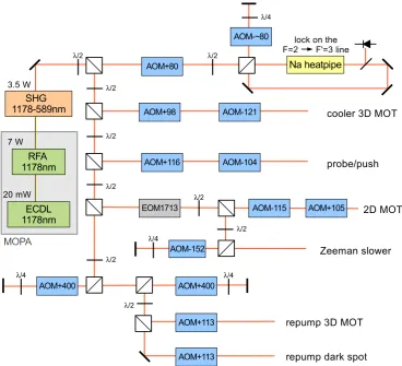
distributed into several beams, each independently controlled in intensity and frequency by means of acousto-optic modulators (AOMs) and electro-optic modulators (EOMs). These devices are located along the path of each beam as indicated in Fig.2.4. For more details on the operative function of
Figure 2.4:Schematic sketch of the optical setup used to produce the light at589nm
needed to laser cool sodium atoms. The lenses used to collimate and to focus the beams are not drawn. The3.5W of light coming out from the duplication cavity
is divided into different beams thanks to thepolarizing beam-splitter(PBS) cubes located on the optical table. These beams can be tuned in frequency using AOMs and EOMs as indicated in the figure.
Each beam is coupled into an optical fiber (SCHAFTER¨ &KIRCHHOFF PMC-630-4.5-NA011-3-APC-900-P) which brings the light from the laser table to the one devoted to the experiment. Each light arm is also equipped with a digitally controlled mechanical shutter (sec.2.5) located in front of the fiber
input. By acting on these shutters it is possible to completely block the yellow light traveling through the fibers up to the experimental table. The typical response time of these devices is∼100ms.
Optical dipole potentials [98], which are obtained from far-detuned laser Optical dipole potentials
light, are used to trap the atoms as well as to change their dynamics. The conservative dipole potential exerted on the atoms can be either attractive (red-detuned light) or repulsive (blue-detuned frequency). The reason of conservativity relies on the low scattering cross-section at sufficiently large detunings, which reduces the heating in the system. Optical potentials can be modeled essentially at will, varying their intensity and geometry.
To obtain the laser radiation needed to create optical potentials, a commer-cial Nd:YAG laser in MOPA configuration (INNOLIGHT MEPHISTO MOPA) is used, providing up to 42 W of light at1064nm. This light presents a
2.3 magnetic fields 29
light can be directly used to generate attractive optical potentials, being red-detuned with respect to theD2atomic transition of sodium.
In addition it is possible to generate repulsive potential since a PP-SLT1
non-linear crystal is placed along the infrared light path. In this case, sending an infrared beam of about30 W trough the crystal produces more than6 W of
green light at a wavelength of532nm. Note that for the work described in
this thesis, the green light at532nm has never been used.
2.3
magnetic fields
To reach quantum degeneracy, the use of magnetic fields is required in or-der to manipulate the neutral atoms. In fact, several magnetic configurations are used during the experimental procedure, for example during the laser cooling stages or to create conservative traps [99].
The very first stages of the experimental sequence (2D-MOT and ZS) re- 2D-MOT and Zeeman Slower
quire a relatively simple magnetic configuration that is obtained using 4
stacks of9neodymium permanent magnets (ECLIPSE N750-RB). These
mag-nets are placed around the HV chamber in order to obtained a quasi-2D
quadrupole. The magnetic field is zero along the unconfined x axis and its modulus varies linearly along the transverse directions. Far from the 2
D-MOT region the magnetic field reaches its maximum, then it decays with the distance. The tails of this vanishing magnetic field are exploited to real-ize the compact ZS [90].
Once that all the atoms are transferred from the HV region to the quartz Driven magnetic electromagnets
cell, the experimental procedure requires a more dynamic control of the magnetic field. This control is achieved thanks to an electric circuit (Fig.2.5)
which controls a set of several coils. These coils are used to generate the magnetic field configurations needed during the experiment. In our experi-mental procedure three main configurations are required:
• MAGNETO-OPTICAL TRAP The experimental sequence starts with a dark spot3D-MOT [100], which is obtained using a quadrupole
mag-netic field, three orthogonal pairs of counter-propagating laser cooling beams and a single "hollow" repumping beam. This beam, which is im-aged on the atomic cloud, is created by means of an8 mm black dot
placed along the beam’s path. The black dot absorbs the light and only the outer profile of the beam is able to pass, so that an hollow Gaussian beam is created.
Before transferring all the atoms to the magnetic trap, a sub-Doppler stage is necessary. This is performed via optical molasses in absence of magnetic fields [101] which leads to almost 3×10⁹ atoms at50 µK. • MAGNETIC TRAP Once that the atoms were sub-Doppler cooled,
they are transferred to a Ioffe–Pitchard conservative magnetic trap (MT) [102]. A confining cigar-shaped potential is then created thanks to the
non-vanishing magnetic field.
• MAGNETIC LEVITATION Since the atomic cloud experiences grav-ity, a procedure to levitate the atoms is often required. In fact this is
crucial to observe atomic expansion or dynamics and to obtain infor-mation about the atom numbers. The atoms’ levitation is obtained via a magnetic field gradient of about8Gcm−1 which is applied along the z direction. In this way the atomic cloud can expand in time-of-flight (TOF) without falling.
Ioffe-Pitchard trap
The Ioffe–Pitchard trap used in the experiment is based on a static magnetic field (presenting a cylindrical symmetry) with a non-zero magnetic field min-imum which prevents from Majorana [103] losses. Along the axial direction
the magnetic field is quadratic with a bias term Bx= B0+B”x2/2. To satisfy
the Maxwell’s equation, the magnetic field in the harmonic approximation must be:
~B(x,y,z) =B0 0 0 1
+B0
x −y 0 + B 00 2 −xz −yz x2− x2+y2
2
. (2.1)
The trapping potential depends only on the modulus of~Band the interac-tion of the atoms with the external magnetic field is given by
U|F,mFi(~r) =µBgFmF|~B(~r)|, (2.2) whereµB is the Bohr magneton,|F,mFidefines the internal Zeeman state
of the atoms andgFis the Landè factor. Considering low-field-seeking states2
and low-temperature regime (µB0 > kBT), the trapping potential can be
approximated to:
U|F,mFi≈ µBgFmFB0+ 1 2mω
2
⊥ y2+z2
+1 2mω
2
xx2. (2.3)
Here the radial trap frequencies and the axial one are respectively ω⊥ =
q
(µat/m)(B 02
B0 −
B00
2 )andωx= p
(µat/m)B00 whereµatis equal to µB|gFmF|.
It is now important to note that for a higher temperature regime the atoms experience a linear confinement along the radial direction that is exploited for evaporative cooling (see sec.3.1).
The value of µBgFmFB0 sets the bottom of the trap and can be changed to
modify the radial confinement and hence the aspect ratio ω⊥/ωx. Electrical circuit and coils
In the experiment the magnetic field minimum of the 3D-MOT and of
the MT are located in the same spatial point so that it is possible to switch from one configuration to the other without moving the atoms. Generally this is not possible since gravity affects the trapping potential displacing its minimum by the so-called gravitational sag∆z= g/ω2z (see Sec.4.2).
The different magnetic configurations described above are obtained using the electrical circuit illustrated in Fig.2.5.
This circuit exploits electro-mechanical relays switches and insulated-gate bipolar transistors (SEMIKRON SKM400GAL12E4). These IGBTs are mainly
2 IfU|
F,mFi(~r)>0 atoms are attracted to the minimum of the potential, ifU|F,mFi(~r)<0 atoms
2.3 magnetic fields 31
Figure 2.5:Scheme of the electric circuit used to generate the magnetic fields needed
to perform all the configurations during the experimental sequence.
used as fast switches, being their response time faster than the relays’ one (1 µs against 10 ms). These devices, however, can also be used as variable
resistors, if driven with an analog voltage. The continuous current flow in the circuit is driven by two power supplies (DELTA ELEKTRONIKA SM30 -200) which can be programmed to provide up to 200A with a maximum
rms-ripple noise of∼20mA.
Figure 2.6:(a) Top view of the main coils used in the experiment. The quadrupole
coils are drawn in azure, the pinch coil in green and the compensations coils in red. In addition the push and the MOT beams are drawn in yellow. (b)3D-view
of the main coils constituting the magnetic circuit of the experiment.
The coils constituting the high-current electrical circuit are shown in Fig.2.6.
In the following, the role of all these coils is explained in detail.
• The quadrupole field used for the dark-spot3D-MOT, as well as for the
MT trap is obtained using a pair of twin coils (azure coils in Fig.2.6) in
anti-Helmholtz3
configuration. Each quadrupole coil is composed of72
windings around an internal radius of5.5cm and are located at±2cm
along the vertical direction (where zero is the center of the MT). The
3 The distance between the center of the two coils is equal to their radius and the current
B0 [G] B0 [G cm−1] B00 [G cm−2] Itot[A]
Iht 3.8 12 118 200
It 1.9 106 59 100
Is 0.9 53 29.5 50
Table 2.1:Trap parameters for the three regimes.
magnetic gradient per units of current produced by the coils in Ioffe– Pitchard configuration is B0/I = 1.06 G/cmA, while the magnetic field curvature is given byB00/I =0.59 G/cm2A.
The atoms’ levitation is obtained by flowing the current in the lower coil only.
• The pinch coil (green coil of Fig.2.6) is activated in the magnetic trap
configuration to create a non-zero magnetic field minimum. It is com-posed of 12 winding around an internal radius of1.3 cm and is 2 cm
![Figure 1.3: Experimental density profiles of the |2, 1⟩ + |1, −1⟩ rubidium mixturetaken from [20]](https://thumb-us.123doks.com/thumbv2/123dok_us/491272.2048201/24.595.200.453.201.401/figure-experimental-density-proles-rubidium-mixturetaken.webp)