Analytical finite element matrix elements and global matrix assembly for hierarchical 3-D vector basis functions within the hybrid finite element boundary integral method

www.adv-radio-sci.net/12/1/2014/ doi:10.5194/ars-12-1-2014

© Author(s) 2014. CC Attribution 3.0 License.

Analytical finite element matrix elements and global matrix

assembly for hierarchical 3-D vector basis functions within the

hybrid finite element boundary integral method

L. Li1, K. Wang1, H. Li2, and T. F. Eibert1

1_{Technische Universität München, Lehrstuhl für Hochfrequenztechnik, Arcisstrasse 21, 80333 Munich, Germany} 2_{Politecnico di Torino, Electronic and Telecommunication, Corso Duca degli Abruzzi, 24, 10129 Torino, Italy} Correspondence to: L. Li ([email protected])

Received: 6 December 2013 – Accepted: 23 January 2014 – Published: 10 November 2014

Abstract. A hybrid higher-order finite element boundary in-tegral (FE-BI) technique is discussed where the higher-order FE matrix elements are computed by a fully analytical pro-cedure and where the gobal matrix assembly is organized by a self-identifying procedure of the local to global trans-formation. This assembly procedure applys to both, the FE part as well as the BI part of the algorithm. The geometry is meshed into three-dimensional tetrahedra as finite elements and nearly orthogonal hierarchical basis functions are em-ployed. The boundary conditions are implemented in a strong sense such that the boundary values of the volume basis func-tions are directly utilized within the BI, either for the tangen-tial electric and magnetic fields or for the asssociated equiv-alent surface current densities by applying a cross product with the unit surface normals. The self-identified method for the global matrix assembly automatically discerns the global order of the basis functions for generating the matrix ele-ments. Higher order basis functions do need more unknowns for each single FE, however, fewer FEs are needed to achieve the same satisfiable accuracy. This improvement provides a lot more flexibility for meshing and allows the mesh size to raise up toλ/3. The performance of the implemented sys-tem is evaluated in terms of computation time, accuracy and memory occupation, where excellent results with respect to precision and computation times of large scale simulations are found.

1 Introduction

The Finite Element Boundary Integral (FE-BI) method (Jin, 2002; Tzoulis and Eibert, 2005; Eibert and Hansen, 1997) is an efficient numerical technique for solving

electromag-netic field problems. Traditional finite element methods rely on utilizing the local information of the FEs. The fixed lo-cal node order forces the lolo-cal matrix elements to be trans-formed into global ones. Facing low order (LO) basis func-tions, the local-global transformation is easy as edge related elements only follow the edge directions. When it comes to higher order (HO) basis functions (Jin, 2002; Sun et al., 2001; Ismatullah and Eibert, 2009; Jorgensen et al., 2004; Graglia et al., 1997; Jorgensen et al., 2005), the basis func-tions are also related to faces, volumes or even more com-plicated structures. The local-global transformation proce-dure introduces then considerably more difficulties. In this paper, a self-identified hierarchical basis function method is illustrated. This method effectively overcomes the problem mentioned above and provides more feasibility within FE-BI. Without fixing the node order or the sequence order of the ba-sis functions for the local FEs, the self-identified hierarchical basis function organization allows a simple assembly of the global equation system. Simultaneously, this method guar-antees the compatibility between FE and BI (Ismatullah and Eibert, 2009) fluently. All arbitrarily shaped components are meshed into tetrahedra (Volakis et al., 1998) apart from per-fect electric conductors (PEC) or perper-fect magnetic conduc-tors (PMC) whereE andH are forced to vanish inside the volume. As FE-BI solves for the field distribution inside the volume together with the corresponding equivalent surface currents (Ismatullah and Eibert, 2009; Rao et al., 1982), the self-identified hierarchical basis functions describe the dis-tribution of fields within the tetrahedra. When observation points tend to the enclosed boundary surface, the boundary condition determines the continuity ofEandH fields (Har-rington, 1961; Bladel, 1964; Mautz and Har(Har-rington, 1978).

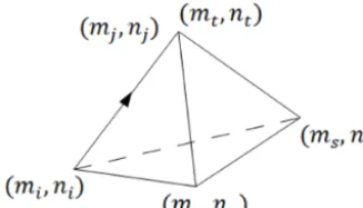
Figure 1. The definition of subscripts based on a single tetrahedron. Every vertex index can be used as a row indexmor as a column indexn.

So it is useful to guarantee that the basis functions for FE are the same as the basis functions for the BI.

Derived from the equivalence theorem, basis functions for BI are used to compose equivalent 2-D surface currents (Rao et al., 1982; Chew et al., 2001; Ylä-Oijala and Taskinen, 2003). The currents are relevant to the surface unit normal vector and the polarization of the fields, thus the tangential component of FE basis functions on the surface is perpen-dicular to the current basis functions. With respect to the cor-responding sources (electric current Js or magnetic current Ms) and the surface normal unit vector, the corresponding

subspaces ensure the compatibility between FE and BI. The LO basis functions have shortcomings when the sim-ulation accuracy and the large number of unknowns are con-sidered. Precision and efficiency of LO are difficult to im-prove with increasing numbers of unknowns. The solution with LO basis functions demands the mesh size to be around λ/20 toλ/8. With coarser meshes, the elements may intro-duce inaccurate waveforms for field reconstruction.

The well-known mixed order basis functions are success-ful for electromagnetic field distributions and surface cur-rent reconstructions. Rao–Wilton–Glisson (RWG) (Rao et al., 1982) basis functions are inherited as LO. As RWG is very effective for BI, it is implemented as the first order of Ro-tational Subspace (0th order) in FE tetrahedra. The Nedelec HO basis functions also form the first order of Gradient Sub-space (1st order), the second order Rotational SubSub-space (2nd order), an so on, where this paper is restricted to 2nd order. Apart from BI, LO and HO basis functions are also utilized within FE and they improve the accuracy for field computa-tions. In FE-BI, 0th and 1st order basis functions for FE and BI are easy to match. Both of them are edge related and fol-low the same direction of the edge vector. The situations for 2nd order basis functions are more complicated. 2nd order basis functions are face related, so that to achieve compati-bility between FE and BI, the basis functions of them have to maintain the same global node order. The tetrahedral FE ba-sis functions defined in Table 1 have a format represented by subscriptsk=(i, j )andk=(r, s, t )as illustrated in Fig. 1. As elements of matrices need row and column positions, the subscripts(mi, mj)and(mr, ms, mt)are introduced for row

basis functions and subscripts (ni, nj)and (nr, ns, nt) are

assigned to column basis functions. In this work,(mi, mj)

and(ni, nj)contain the global order of local node numbers

for edge related basis functions, whereas (mr, ms, mt) and (nr, ns, nt)represent the global order of nodes for face

re-lated basis functions, wherek=(i, j )andk=(r, s, t )store the local node number of finite elements.

In FE analysis, the self-identified hierarchical basis func-tions are derived from the geometrical information of the tetrahedra. In the mesh file, the data structure for each tetra-hedra contains six edge identities and four face identities. Each edge is constructed with two node numbers and the order of the two nodes determines the edge global direc-tion. Every face has the identity of the corresponding out-side boundary triangles, inout-side volume triangles or inout-side boundary triangles. The outside boundary triangles are de-scribed by three edges in certain directions. The first edge gives out the first two nodes of the outside boundary trian-gle, the last node can be found through another two edges. The order of these three nodes are inherited as global node order. The inside volume triangles and inside boundary tri-angles are constructed by three nodes directly and the node order is viewed as the global node order. Through the in-dex of edge and face identities, the tetrahedral FEs can easily consult the corresponding edges and triangles. Thus the de-termined global node order can be set for the LO and HO ba-sis functions. As shown in Fig. 1,(mi, ni)always represent

the starting point of the edge,(mj, nj)represent the ending

point and(mr, nr),(ms, ns),(mt, nt)represent the node

or-der of the triangle. Practically, the local node numbers are arrayed in the unique global order and assigned to the corre-sponding subscripts. When generating the system matrices, the assigned subscripts are set to the corresponding positions into the list of basis functions. Thus elements of system ma-trices are automatically assigned to global edges and faces. If HO basis functions are implemented into FE, the matrix elements can be calculated analytically and precisely. Since these results are commonly not available in FE literature, it is a major contribution of this paper to present these analyt-ical matrix elements up to 2nd order. As the order of basis functions is enlarged, the accuracy of the boundary integral (BI) should also be improved. As it turns out, the integration order for the testing surface integrals should be increased, the adaptive numbers of quadrature points in the singular-ity cancellation technique have to grow and larger maximum numbers for spherical harmonic expansion terms are needed within the Multilevel Fast Multipole Method (Eibert, 2005).

more accurate, so that the flexibility of mesh size provided by HO gives a more feasible solution. Meanwhile, HO improves the accuracy and also reduces the number of finite elements. FE-BI solutions for coated spheres and the Flamme air-craft referring to the self-identified hierarchical nearly or-thogonal basis functions are explicitly illustrated. The ma-terial of the layered sphere is homogeneous, isotropic and lossy. A variety of FE-BI simulations up to 3 million un-knowns based on self-identified hierarchical basis functions are presented. The accuracy of HO testing cases is good, and the simulation results based on HO basis functions are also compared with LO situations.

2 Finite element variational formulation

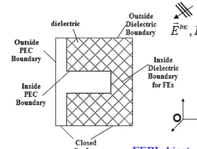
Consider the configuration of an arbitrary volume as shown in Fig. 2. A typical FE model consists of a finite volumeVa

with possibly anisotropic and inhomogeneous materials in-side. The materials are characterized by relative permittivity ↔

r(r)and relative permeability

↔

µr(r).Ad is the assembled

enclosed envelope and_bn(r)is the normal vector pointing out ofVa.

Assuming a field expansion E=P

unαn and H=

P

inαnas well as a suppressed time dependenceej ωt, a

lin-ear system of equations (Jin, 2002; Tzoulis and Eibert, 2005) is achieved as

([Rmn]−k20[Smn])[un]+j k0Z0[Tmn][in]=−j k0Z0[wm]. (1)

The system matrices [Rmn], [Smn], [Tmn] and the right hand

side vector [w_m] are defined as [Rmn]=

Z Z Z

Va

{∇×am(r)·

↔

µr−1(r)·∇×an(r)}dv, (2)

[Smn]=

Z Z Z

Va

{am(r)·

↔

r(r)·an(r)}dv, (3)

[Tmn]=

ZZ

Ad

am(r)·(an(r)×bn(r))da, (4)

[wm]=

Z Z Z

Va

{am(r)·Jd(r)}dv, (5)

where am and an are field basis functions, k0=ω

√ 0µ0 is the free space wave number, Z0=

√

µ0/0 is the free space intrinsic impedance, andJd is a volume current

den-sity source.

The hierarchical basis functions are based on the nor-malized barycentric (simplex) coordinates in FE tetrahedra (λ0, λ1, λ2, λ3), whereλ0+λ1+λ2+λ3=1. The functions are also related to the gradients ∇λi(i=0,1,2,3)and the

volume of the tetrahedron VT. Equation (2) is related to

the curl of the basis functions. Equations (2) and (3) form the system matrices related to electric field unknowns [un].

Figure 2. The general geometrical configuration for finite element– boundary integral method.

Equation (4) generates the matrices related to surface mag-netic field unknowns [in] where the integral region is the

en-velope ofVa. Equation (5) is related to the current excitation

inside the volume. AsVa=PVe andAd=PAe,

integra-tion intervals of Eqs. (2), (3), (4) and (5) are the combinaintegra-tion of finite elements. With simplex coordinates, the properties of basis functions allow for an analytical solution of the ma-trices in Eq. (1).

3 3-D HO self-identified basis functions

The general format of FE-BI basis functions for different orders is displayed in Table 1.Ai (i=0,1,2,3)is the

lo-cal face area vector related to surfaces of the tetrahedron pointing into the volume,VT is the tetrahedral volume. Face

vectors are independent in the tetrahedron and the surface tangential part of field basis functions compared with sur-face current basis functions are perpendicular. The field basis functions distribute inside the finite element volume. When tending to the tetrahedral boundary edges and faces, the cor-responding tangential parts of edge basis functions for 0th and 1st order exist on the adjacent connected surfaces, they are zero on other edges or faces. The tangential components of face based functions for 2nd order only exist on the related face, but vanish on the other unrelated faces and on all edges. The compatibility between FE and BI is easily achieved by utilizing self-identified hierarchical bases defined by global node order. The identified hierarchical basis functionsαi are

composed of rotational first order (0th order) represented by

a1, gradient first order (1st order) represented byb1and ro-tational second order (2nd order) related toc2andd2. Prop-erties of identified hierarchical basis functions are displayed in Table 1.(i, j )and(r, s, t )in Table 1 contain the local node numbers in the series defined by global order. Also, the curl of identified hierarchical basis functions is given.

4 Analytical calculation of FE system matrices

With self-identified hierarchical basis functions, analytical solutions for system matrices can be achieved through the properties of simplex coordinates in tetrahedra. The inner products of simplex coordinates (Lapidus and Pinder, 1982) are given as

L2(λp;λq)=

Z Z Z

VT

λpλqdv=6VT X!

5!

X=

(

2, p=q

1, p6=q,{p, q} = {0,1,2,3}, (6)

L3(λr;λp, λq)=

Z Z Z

VT

λrλpλqdv=6VT X!

6!

X=

(

2, r=p, q

1, r6=p, q,{r, p6=q} = {0,1,2,3}, (7)

L4(λr, λs;λp, λq)=

Z Z Z

VT

λrλsλpλqdv=6VT X!Y!

7!

X=

(

2, r=p, q

1, r6=p, q,{r, p6=q} = {0,1,2,3} Y=

(

2, s=p, q

1, s6=p, q,{s, p6=q} = {0,1,2,3}. (8) The dot and cross products between face vectors are defined as

Ipq=Ap·Aq,{p6=q} = {0,1,2,3}, (9)

Tpq=Ap×Aq,{p6=q} = {0,1,2,3}. (10)

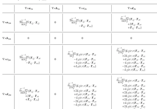
Combining identified basis functions and their properties (Table 1, Eqs. 6–10), the system matrix[Rmn]is calculated in

Table 2 and[Smn]is given in Table 3. From Eqs. (2) and (3),

matrices[Rmn]and[Smn]are symmetric, so that the elements

at symmetric positions in Tables 2 and 3 are identical and it is explicit that the functions are the same along columns and rows.

System matrices [Tmn] depend on the surface boundaries

of the volume, so that the dimension of the hierarchical space is reduced. In fact Eq. (4) can be written as

[Tmn]=

ZZ

Ad

(am(r)×an(r))·bn(r))da, (11)

and the hierarchical space turns out to be

as=λi∇λj−λj∇λi =

1 2AT

(λilj−λjli)

{i, j} = {1,2,3},{i < j}, (12)

bs=λi∇λj+λj∇λi=

1 2AT

(λilj+λjli)

{i, j} = {1,2,3},{i < j}, (13)

cs=λrλs∇λt+λsλt∇λr−2λrλt∇λs = 1

2AT

(λrλslt+λsλtlr−2λrλtls)

{r, s, t} = {1,2,3},{r < s < t}, (14)

ds=λrλs∇λt−λsλt∇λr

= 1 2AT

(λrλslt−λsλtlr)

{r, s, t} = {1,2,3},{r < s < t}. (15) With properties of surface triangle finite elements (Lapidus and Pinder, 1982), it is shown that

Z Z

AT λm1

1 λ

m2 2 λ

m3

3 da=2AT

m1!m2!m3!

(m1+m2+m3+2)!

, (16)

li×lj= −2AT(−1)j−i,{i < j}, (17) A_T =1

2t12×t13. (18)

Based on Eq. (11), [Tmn] is computed as

[Tmn]=

Z Z

AT

{[as,bs,cs,ds]T×[as,bs,cs,ds]·bn(r)}da

=1

6[cnA·bn(r)]·



          

0 1 1 −1/2 1/2 1/2 1/4 1/4 −1 0 1 −1/2 1/2 −1/2 1/2 0 −1 −1 0 1/2 1/2 −1/2 1/4 −1/4 1/2 1/2 −1/2 0 0 0 −3/20 1/20 −1/2 −1/2 −1/2 0 0 0 0 −1/10 −1/2 1/2 1/2 0 0 0 3/20 1/20 −1/4 −1/2 −1/4 3/20 0 −3/20 0 −1/10 −1/4 0 1/4 −1/20 1/10 −1/20 1/10 0



           .

(19) From Eq. (5), [wm] can be written as

[wm] =

Z Z Z

VT

          

a1

b1

c2

d2

   

·Jd

      

dv, (20)

where the current source Jd can be used directly for the

product with self-identified 3-D basis functions and vector [wm] can be easily solved.

Table 1. Hierarchical basis functions and properties within the tetrahedron (Sun et al., 2001).

FE Vector Basis Functionsαi ∇ ×αi

R1 a1 λi∇λj−λj∇λi λiAj₃−_VλjAi

T 2

∇λi× ∇λj

2

9V_T2(Ai×Aj)

G1 b1 λi∇λj+λj∇λi λiAj₃+_VλjAi

T 0 0

R2 c₂

λrλs∇λt

+λsλt∇λr

−2λrλt∇λs

λrλsAt+λsλtAr−2λrλtAs 3VT

3λr∇λs× ∇λt

−3λt∇λr× ∇λs

1

3V_T2(λrAs×At

−λtAr×As)

d2 λrλs ∇λt

−λsλt∇λr

λrλsAt−λsλtAr 3VT

λr∇λs× ∇λt

+2λs∇λr× ∇λt

+λt∇λr× ∇λs

1

9V_T2(λrAs×At

+2λsAr×At

+λtAr×As)

Table 2. Analytical solution for[Rmn]matrix elements.

∇×a1n ∇×b1n ∇×c2n ∇×d2n

∇×a_1m 4

↔

µr

−1

(r)

81V3 T

Tij·Tij 0

4µ↔r

−1

(r)

81V_T3 {Tij·Tst

−Tij·Trs}

↔

µr

−1

(r)

162V_T3 {Tij·Tst

+2Tij·Trt

+T_ij·Trs}

∇×b_1m 0 0 0 0

∇×c2m

4µ↔r

−1

(r)

81V_T3 {Tij·Tst

−T_ij·Trs}

0

↔

µr

−1

(r)

9V_T4 {L2(r;r)Tst·Tst

−L2(r;t )Tst·Trs

−L2(t;r)Trs·Tst

+L2(t;t )Trs·Trs}

↔

µr

−1

(r)

27V_T4 {L2(r;r)Tst·Tst

+2L2(r;s)Tst·Trt

+L2(r;t )Tst·Trs

−L2(t;r)Trs·Tst

−2L2(t;s)Trs·Trt

−L2(t;t )Trs·Trs}

∇×d2m

↔

µr

−1

(r)

162V_T3 {Tij·Tst

+2T_ij·Trt

+Tij·Trs}

0

↔

µr

−1

(r)

27V_T4 {L2(r;r)Tst·Tst

+2L2(r;s)Tst·Trt

+L2(r;t )Tst·Trs

−L2(t;r)Trs·Tst

−2L2(t;s)Trs·Trt

−L2(t;t )Trs·Trs}

↔

µr

−1

(r)

81V4 T

{L2(r;r)Tst·Tst

+2L2(r;s)Tst·Trt

+L2(r;t )Tst·Trs

+2L2(s;r)Trt·Tst

+4L2(s;s)Trt·Trt

+2L2(s;t )Trt·Trs

+L2(t;r)Trs·Tst

+2L2(t;s)Trs·Trt

+L2(t;t )Trs·Trs}

Table 3. Analytical solution for[Smn]matrix elements.

a1n b1n c2n d2n

a1m

↔

r(r)

9V_T2{L2(i;i)Ijj

−L2(i;j )Ij i

−L2(j;i)Iij

+L2(j;j )Iii}

↔

r(r)

9V_T2{L2(i;i)Ijj

+L2(i;j )Ij i

−L2(j;i)Iij

−L2(j;j )Iii}

↔

r(r) 9V2

T

{L3(i;r, s)Ij t

+L3(i;s, t )Ij r

−2L3(i;r, t )Ij s

−L3(j;r, s)Iit

−L3(j;s, t )Iir

+2L3(j;r, t )Iis}

↔

r(r)

9V_T2{L3(i;r, s)Ij t

−L3(i;s, t )Ij r

−L3(j;r, s)Iit

+L3(j;s, t )Iir}

b_1m

↔

r(r)

9V_T2{L2(i;i)Ijj

+L2(i;j )Ij i

−L2(j;i)Iij

−L2(j;j )Iii}

↔

r(r)

9V_T2{L2(i;i)Ijj

+L2(i;j )Ij i

+L2(j;i)Iij

+L2(j;j )Iii}

↔

r(r)

9V_T2{L3(i;r, s)Ij t

+L3(i;s, t )Ij r

−2L3(i;r, t )Ij s

+L3(j;r, s)Iit

+L3(j;s, t )Iir

−2L3(j;r, t )Iis}

↔

r(r)

9V_T2{L3(i;r, s)Ij t

−L3(i;s, t )Ij r

+L3(j;r, s)Iit

−L3(j;s, t )Iir}

c2m

↔

r(r) 9V2

T

{L3(i;r, s)Ij t

+L3(i;s, t )Ij r

−2L3(i;r, t )Ij s

−L3(j;r, s)Iit

−L3(j;s, t )Iir

+2L3(j;r, t )Iis}

↔

r(r) 9V2

T

{L3(i;r, s)Ij t

+L3(i;s, t )Ij r

−2L3(i;r, t )Ij s

+L3(j;r, s)Iit

+L3(j;s, t )Iir

−2L3(j;r, t )Iis}

↔

r(r)

9V_T2{L4(r, s;r, s)It t

+L4(r, s;s, t )It r

−2L4(r, s;r, t )It s

+L4(s, t;r, s)Irt

+L4(s, t;s, t )Irr

−2L4(s, t;r, t )Irs

−2L4(r, t;r, s)Ist

−2L4(r, t;s, t )Isr

+4L4(r, t;r, t )Iss}

↔

r(r) 9V2

T

{L4(r, s;r, s)It t

−L4(r, s;s, t )It r

+L4(s, t;r, s)Irt

−L4(s, t;s, t )Irr

−2L4(r, t;r, s)Ist

+2L4(r, t;s, t )Isr}

d2m

↔

r(r)

9V_T2{L3(i;r, s)Ij t

−L3(i;s, t )Ij r

−L3(j;r, s)Iit

+L3(j;s, t )Iir}

↔

r(r)

9V_T2{L3(i;r, s)Ij t

−L3(i;s, t )Ij r

+L3(j;r, s)Iit

−L3(j;s, t )Iir}

↔

r(r)

9V_T2{L4(r, s;r, s)It t

−L4(r, s;s, t )It r

+L4(s, t;r, s)Irt

−L4(s, t;s, t )Irr

−2L4(r, t;r, s)Ist

+2L4(r, t;s, t )Isr}

↔

r(r)

9V_T2{L4(r, s;r, s)It t

−L4(r, s;s, t )It r

−L4(s, t;r, s)Irt

+L4(s, t;s, t )Irr}

5 Surface integral formulation

With Huygen’s principle (Ismatullah and Eibert, 2009; Har-rington, 1961; Chew et al., 2001), the radiation sources can be replaced by equivalent electric surface currents Js

and magnetic surface currents Ms on the volume enclosed

boundaryAd for evaluation of free space radiation. The

nu-merical solution for the surface currents are based on the well known EFIE, MFIE and CFIE (Ismatullah and Eibert, 2009; Rao et al., 1982; Ylä-Oijala and Taskinen, 2003), given as

EF I E:1

2Ms+bn×[3(Ms)+Z0K(Js)]=−bn×E

inc_{, (21)}

MF I E:1 2Js+bn×

3(Js)−

1 Z0

K(Ms)

=

bn×H

inc_{, (22)}

CF I E: αEF I E+Z0(1−α)bn×MF I E, (23)

L. Li et al.: Finite element matrix for hierarchical basis functions 7

6

Li Li et al.: Finite element matrix for hierarchical basis functions

and fully staffed,

M

i

is square, symmetrical and fully

oc-355

cupied,

V

_{are excitation vectors for FE-BI. Thus, the}

complete combined system is written as

M

M

M

M

u

i

=

V

V

.

(31)

The complete system solves the electric and magnetic fields

360

simultaneously, thus equivalent surface electric and magnetic

currents can be achieved.

7

Numerical Results

To testify the accuracy of the analytical matrix elements

and the global matrix assembly in FE-BI, several numerical

365

simulation results are shown in this section. A cogent

demon-stration is to utilize a coated sphere testing case, where a PEC

sphere is enclosed by a layer of dielectric material. The

ana-lytical RCS is well known as MIE Scattering (C. A. Balanis

(1989)). Good matching of RCS between analytical solution

370

and numerical method verifies the efficacy of FE-BI. As a

more complicated testing case, a second sphere is displayed.

With higher frequency and finer mesh, more unknowns are

handled. Moreover, an example of FE-BI application in very

large scale simulations is shown through the RCS of the

375

Flamme aircraft. As 0th order of FE-BI has been verified in

many published articles (A. Tzoulis and T. F. Eibert (2005);

T. F. Eibert and V. Hansen (1997); T. F. Eibert (2007)), it can

be utilized as a reference for HO BI. Efficiency of

FE-BI based on different orders of self-identified basis functions

380

are presented. The sphere simulations were performed on a

PC with Intel(R) Core(TM)2 Quad CPU Q9550 @ 2.83 GHz

processor, installed memory (RAM) 16.0 GB and 64-bit

op-erating system. The simulation of the Flamme aircraft was

operated on a Server with Intel(R) Xeon(R) CPU E5630 @

385

2.53 GHz (2 processors), installed memory (RAM) 96.0 GB

and 64-bit operating system. All simulations were computed

on one core.

7.1

Coated Sphere I

For the coated sphere, the RCS from 0th, 1st and 2nd

or-390

der of self-identified basis functions for FE-BI are compared

with MIE scattering as shown in Fig. 3. The coated sphere

consists of a PEC core with radius 0.9 m and a layer of

di-electrics with thickness 0.1 m. The dielectric layer properties

are given by

ǫ

= 3

−

0

.

1

j

and

µ

= 1

.

0

. The incident wave

395

is 550 MHz and propagating towards

+

z

direction and the

electric field is 100 V/m along

x

direction (E

= 100

V/m).

For 0th order, the mesh size was set to 0.04 m in

Hy-permesh software (HyperWorks (2012)), and the mean edge

length is 4.65 cm, with minimum edge length 2.24 cm and

400

maximum edge length 8.11 cm. The total unknowns are

154 822. The running time was 1 314.8 s. For 1st order, the

same mesh as for 0th order was utilized. The total unknowns

0 10 20 30

0 30 60 90 120 150 180

B is ta tic R C S in d B sm

Azimuth angleϑin deg

MIE Scattering

0th Order 1st Order 2nd Order

Fig. 3.Bistatic RCS ofCoated Sphere I@550 MHz onxzcut half plane (ϕ= 0◦_).

are 309 644. The running time was 4 763.4 s. For 2nd

or-der, the mesh size is set 0.1 m, and the mean edge length

405

is 10.93 cm, with minimum edge length 6.48 cm and

maxi-mum edge length 18.08 cm. The total unknowns are 70 448.

The running time was 419.6 s.

The mesh size of LO is around

λ/

8

and the mesh size

of HO is enlarged up to around

λ/

3

. HO with coarser mesh

410

and fewer unknowns achieves also accurate result as LO with

finer mesh.

7.2

Coated Sphere II

For the second coated sphere testing case, numerical RCS

from different orders are also compared with MIE scattering.

415

The second coated sphere contains a PEC sphere core with

radius 0.5 m, and the PEC core is enclosed with a dielectric

layer with thickness 0.0025 m. The properties of the

dielec-tric layer are presented with

ǫ

= 2

.

5

−

0

.

5

j

and

µ

= 1

.

0

.

The incident wave is 3 GHz and propagating toward

+

z

di-420

rection and the electric field is 100 V/m along

x

direction

(E

= 100

V/m). The results for the RCS are shown in Fig. 4.

−25 −15 −5 5 15 25 35

0 30 60 90 120 150 180

B is ta tic R C S in d B sm

Azimuth angleϑin deg MIE Scattering 0th Order–finer mesh 1st Order–finer mesh 2nd Order–finer mesh 2nd Order–coarser mesh

Fig. 4.Bistatic RCS ofCoated Sphere II@3 GHz onxz cut half plane (ϕ= 0◦_).

Figure 3. Bistatic RCS of Coated Sphere I @ 550 MHz onxzcut half plane (ϕ=0◦).

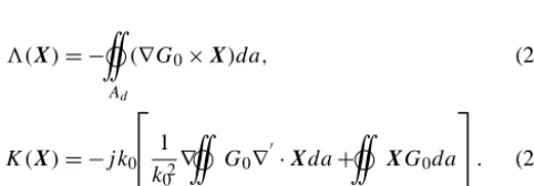
3(X)= −

ZZ

Ad

(∇G0×X)da, (24)

K(X)= −j k0

  

1 k02

∇

ZZ

Ad G0∇

0

·Xda+

ZZ

Ad

XG0da

 

. (25)

EincandHincare incident electric and magnetic fields,G0 is the scalar Green’s function in free space andαis a number between zero and one.JsandMs are given as

Js =bn×H, Ms= −bn×E. (26)

Thus the electric and magnetic currents can be written as

Js =

X

inbn×an, Ms= − X

unbn×an. (27)

Withfn=bn×an(Ylä-Oijala and Taskinen, 2003),Js and

Ms are expanded as

Js = NI

X

n=1

infn, Ms= − NM

X

n=1

unfn, (28)

wherefn is the 2-D surface hierarchical basis function for

BI, in and un in Eq. (27) are coefficients with respect to

the surface elements and the total number of BI unknowns isN=NI+NM.

The discretized solution for MoM can be achieved through Galerkin’s process and fast solutions as given by (Ismatul-lah and Eibert, 2009, 2008; Notaros, 2002; Eibert, 2005; No-taros, 2008) can be utilized. The definition of HO fn is in

2-D derived from 3-D HOan, thus the system matrices from

MoM and FE will be compatible based on the same geomet-rical structure information of the object. The system matrices from BI are described in Ismatullah and Eibert (2009). and fully staffed,MBI

i is square, symmetrical and fully

oc-355

cupied,VF E,BI _{are excitation vectors for FE-BI. Thus, the}

complete combined system is written as

MF E u MiF E MBI

u MiBI

u i =

VF E VBI

. (31)

The complete system solves the electric and magnetic fields 360

simultaneously, thus equivalent surface electric and magnetic currents can be achieved.

7 Numerical Results

To testify the accuracy of the analytical matrix elements and the global matrix assembly in FE-BI, several numerical 365

simulation results are shown in this section. A cogent demon-stration is to utilize a coated sphere testing case, where a PEC sphere is enclosed by a layer of dielectric material. The ana-lytical RCS is well known as MIE Scattering (C. A. Balanis (1989)). Good matching of RCS between analytical solution 370

and numerical method verifies the efficacy of FE-BI. As a more complicated testing case, a second sphere is displayed. With higher frequency and finer mesh, more unknowns are handled. Moreover, an example of FE-BI application in very large scale simulations is shown through the RCS of the 375

Flamme aircraft. As 0th order of FE-BI has been verified in many published articles (A. Tzoulis and T. F. Eibert (2005); T. F. Eibert and V. Hansen (1997); T. F. Eibert (2007)), it can be utilized as a reference for HO BI. Efficiency of FE-BI based on different orders of self-identified basis functions 380

are presented. The sphere simulations were performed on a PC with Intel(R) Core(TM)2 Quad CPU Q9550 @ 2.83 GHz processor, installed memory (RAM) 16.0 GB and 64-bit op-erating system. The simulation of the Flamme aircraft was operated on a Server with Intel(R) Xeon(R) CPU E5630 @ 385

2.53 GHz (2 processors), installed memory (RAM) 96.0 GB and 64-bit operating system. All simulations were computed on one core.

7.1 Coated Sphere I

For the coated sphere, the RCS from 0th, 1st and 2nd or-390

der of self-identified basis functions for FE-BI are compared with MIE scattering as shown in Fig. 3. The coated sphere consists of a PEC core with radius 0.9 m and a layer of di-electrics with thickness 0.1 m. The dielectric layer properties are given byǫr= 3−0.1jandµr= 1.0. The incident wave

395

is 550 MHz and propagating towards+z direction and the electric field is 100 V/m alongxdirection (Ex= 100V/m).

For 0th order, the mesh size was set to 0.04 m in Hy-permesh software (HyperWorks (2012)), and the mean edge length is 4.65 cm, with minimum edge length 2.24 cm and 400

maximum edge length 8.11 cm. The total unknowns are 154 822. The running time was 1 314.8 s. For 1st order, the same mesh as for 0th order was utilized. The total unknowns

0 10 20 30

0 30 60 90 120 150 180

B is ta tic R C S in d B sm

Azimuth angleϑin deg

MIE Scattering 0th Order 1st Order 2nd Order

Fig. 3.Bistatic RCS ofCoated Sphere I@550 MHz onxzcut half plane (ϕ= 0◦_).

are 309 644. The running time was 4 763.4 s. For 2nd or-der, the mesh size is set 0.1 m, and the mean edge length 405

is 10.93 cm, with minimum edge length 6.48 cm and maxi-mum edge length 18.08 cm. The total unknowns are 70 448. The running time was 419.6 s.

The mesh size of LO is around λ/8 and the mesh size of HO is enlarged up to aroundλ/3. HO with coarser mesh 410

and fewer unknowns achieves also accurate result as LO with finer mesh.

7.2 Coated Sphere II

For the second coated sphere testing case, numerical RCS from different orders are also compared with MIE scattering. 415

The second coated sphere contains a PEC sphere core with radius 0.5 m, and the PEC core is enclosed with a dielectric layer with thickness 0.0025 m. The properties of the dielec-tric layer are presented withǫr= 2.5−0.5j and µr= 1.0.

The incident wave is 3 GHz and propagating toward+z di-420

rection and the electric field is 100 V/m alongx direction (Ex= 100V/m). The results for the RCS are shown in Fig. 4.

−25 −15 −5 5 15 25 35

0 30 60 90 120 150 180

B is ta tic R C S in d B sm

Azimuth angleϑin deg MIE Scattering 0th Order–finer mesh 1st Order–finer mesh 2nd Order–finer mesh 2nd Order–coarser mesh

Fig. 4.Bistatic RCS ofCoated Sphere II@3 GHz onxzcut half plane (ϕ= 0◦_).

Figure 4. Bistatic RCS of coated sphere II @ 3 GHz onxzcut half plane (ϕ=0◦).

6 Linear algebraic equation system

To solve the electric field [u] and the magnetic field [i], the subsystem from FE in form of Eq. (1) and the subsystem gen-erated by BI (Ismatullah and Eibert, 2009) must be combined as a complete system. The BI subsystem based on EFIE may introduce resonances into the final system, so it is necessary to utilize CFIE with similarly satisfiable accuracy. As a re-sult, the subsystems can be regarded as

M_uFE[u]+M_iFE[i]=VFE, (29)

M_uBI[u]+M_iBI[i]=VBI, (30) where M_u,iFE,BI is the sub-matrix derived from FE-BI for corresponding u and i. M_uFE is square, symmetrical and sparse,M_iFEis rectangular and sparse,M_uBIis rectangular and fully staffed,M_iBIis square, symmetrical and fully occupied, VFE,BIare excitation vectors for FE-BI. Thus, the complete combined system is written as

M_uFE M_iFE M_uBI M_iBI

u i = VFE VBI . (31)

The complete system solves the electric and magnetic fields simultaneously, thus equivalent surface electric and magnetic currents can be achieved.

7 Numerical results

To testify the accuracy of the analytical matrix elements and the global matrix assembly in FE-BI, several numerical sim-ulation results are shown in this section. A cogent demon-stration is to utilize a coated sphere testing case, where a PEC sphere is enclosed by a layer of dielectric material. The analytical RCS is well known as MIE Scattering (Balanis, 1989). Good matching of RCS between analytical solution

Figure 5. The geometry of a Flamme airplane.

and numerical method verifies the efficacy of FE-BI. As a more complicated testing case, a second sphere is displayed. With higher frequency and finer mesh, more unknowns are handled. Moreover, an example of FE-BI application in very large scale simulations is shown through the RCS of the Flamme aircraft. As 0th order of FE-BI has been verified in many published articles (Tzoulis and Eibert, 2005; Eib-ert and Hansen, 1997; EibEib-ert, 2007), it can be utilized as a reference for HO FE-BI. Efficiency of FE-BI based on dif-ferent orders of self-identified basis functions are presented. The sphere simulations were performed on a PC with In-tel(R) Core(TM)2 Quad CPU Q9550 @ 2.83 GHz proces-sor, installed memory (RAM) 16.0 GB and 64-bit operating system. The simulation of the Flamme aircraft was operated on a Server with Intel(R) Xeon(R) CPU E5630 @ 2.53 GHz (2 processors), installed memory (RAM) 96.0 GB and 64-bit operating system. All simulations were computed on one core.

7.1 Coated sphere I

For the coated sphere, the RCS from 0th, 1st and 2nd order of self-identified basis functions for FE-BI are compared with MIE scattering as shown in Fig. 3. The coated sphere consists of a PEC core with radius 0.9 m and a layer of dielectrics with thickness 0.1 m. The dielectric layer properties are given by r=3−0.1j andµr=1.0. The incident wave is 550 MHz

and propagating towards+zdirection and the electric field is 100 V/m alongxdirection (Ex=100 V/m).

For 0th order, the mesh size was set to 0.04 m in Hy-permesh software (HyperWorks, 2012), and the mean edge length is 4.65 cm, with minimum edge length 2.24 cm and maximum edge length 8.11 cm. The total unknowns are 154 822. The running time was 1314.8 s. For 1st order, the same mesh as for 0th order was utilized. The total unknowns are 309 644. The running time was 4763.4 s. For 2nd or-der, the mesh size is set 0.1 m, and the mean edge length is 10.93 cm, with minimum edge length 6.48 cm and maximum

Figure 6. Bistatic RCS of Flamme @ 2.5 GHz onxycut plane (ϑ= 90◦).

edge length 18.08 cm. The total unknowns are 70 448. The running time was 419.6 s.

The mesh size of LO is around λ/8 and the mesh size of HO is enlarged up to aroundλ/3. HO with coarser mesh and fewer unknowns achieves also accurate result as LO with finer mesh.

7.2 Coated sphere II

For the second coated sphere testing case, numerical RCS from different orders are also compared with MIE scattering. The second coated sphere contains a PEC sphere core with radius 0.5 m, and the PEC core is enclosed with a dielectric layer with thickness 0.0025 m. The properties of the dielec-tric layer are presented withr =2.5−0.5j andµr=1.0.

The incident wave is 3 GHz and propagating toward+z di-rection and the electric field is 100 V/m along x direction (Ex=100 V/m). The results for the RCS are shown in Fig. 4.

For 0th order, the mesh size was set to 0.01 m, and the mean edge length is 0.858 cm, with minimum edge length 0.250 cm and maximum edge length 1.631 cm. The total un-knowns are 411 339. The running time was 3525.6 s. For 1st order, the same mesh as 0th order is utilized. The total un-knowns are 822 678. The running time was 4271.3 s. For 2nd order, there are two testing cases. One uses the same mesh as 0th and 1st order. The total unknowns are 1 973 604. The running time was 7725.5 s. Another simulation utilizes mesh size 0.03 in Hypermesh, and the mean edge length is 2.554 cm. The minimum edge is 0.250 cm and maximum edge length 4.316 cm. The total unknowns are 202 522. The running time was 1357.6 s.

Figure 7. Bistatic RCS of Flamme @ 2.5 GHz onxzcut half plane (ϕ=0◦).

Figure 8. Bistatic RCS of Flamme @ 2.5 GHz onyzcut half plane (ϕ=90◦).

settled. When the mesh size of HO increases up to around λ/4, HO with coarser mesh for FE-BI maintains good pre-cision as the results from LO with finer mesh as shown in Fig. 4.

7.3 Flamme

The Flamme case is an application of FE-BI for very large scale simulation. The Flamme is located in thexyplane, with nose heading along the +x axis, as shown in Fig. 5. The Flamme is enclosed by a layer of lossy dielectric material with thickness of approximately 1 cm. The permittivity of the dielectric material isr =1.21−10j and the permeability is µr=1. The simulation frequency is 2.5 GHz. The incident

plane wave propagates towards −x direction, with electric

Figure 9. Bistatic RCS of Flamme @ 2.5 GHz onxzcut half plane (ϕ=180◦).

Figure 10. Bistatic RCS of Flamme @ 2.5 GHz onyzcut half plane (ϕ=270◦).

field (Ez=100 V/m). To visualize absorbing effects of the

lossy dielectric material, a PEC Flamme simulated with BI with 0th order of basis functions is utilized for comparison.

The RCS of PEC and layered Flamme in different cut planes are shown in Figs. 6–10. The PEC Flamme is simu-lated through BI with 0th order of self-identified basis func-tions, the layered Flamme is simulated through FE-BI with 0th, 1st and 2nd order of self-identified basis functions. As the efficacy of 0th order with finer mesh has been verified, here it is used as a reference. The RCS comparison shows that most of input power goes over the Flamme. In scattered directions, the scattered power is evidently absorbed by the dielectric material. Figure 11 shows the equivalent surface electric current of the covered Flamme.

Figure 11. Electric surface current density |J| in A/m distribu-tion of a covered Flamme airplane with plane wave incidence @ 2.5 GHz.

For PEC, the mesh size of the PEC Flamme was set to 0.01 m, and the mean edge length is 1.011 cm, with minimum edge length 0.100 cm and maximum edge length 2.559 cm. The total unknowns are 692 952. The number of BI elec-tric currents is 692 952 and the number of BI magnetic cur-rents is 0. The number of levels for MLFMM is 8 and the peak memory consumption was 4083.746 MBytes. The run-ning time was 75 529.3 s. For 0th order, the mesh size of the layered Flamme was set to 0.01 m, and the mean edge length is 1.083 cm, with minimum edge length 0.044 cm and maximum edge length 2.671 cm. The total unknowns are 2 081 547. The number of BI electric currents is 690 960 and the number of BI magnetic currents is 602 284. The number of levels for MLFMM is 8 and the peak memory consump-tion was 11 384.43 MBytes. The run time was 23 511.6 s. For 1st order, the mesh size of layered Flamme was set to 0.02 m, the mean edge length is 1.770 cm, with minimum edge length 0.065 cm and maximum edge length 3.933 cm. The total un-knowns are 1 252 430. The number of BI electric currents is 427 144 and the number of BI magnetic currents is 360 976. The number of levels for MLFMM is 7 and the peak memory consumption was 8825.734 MBytes. The running time was 12 141.3 s. For 2nd order, the mesh size was set to 0.02 m, and the mean edge length is 1.770 cm, with minimum edge length 0.065 cm and maximum edge length 3.933 cm. The total unknowns are 2 941 242. The number of BI electric cur-rents is 712 284 and the number of BI magnetic curcur-rents is 602 004. The number of levels for MLFMM is 8 and the peak memory consumption was 18 536.68 MByte. The run-ning time was 47 871.3 s.

8 Conclusion

Self-identified hierarchical 3-D vector basis functions were generated for the hybrid finite element (FE) – boundary integal (BI) technique, where analytical solutions for the FE matrix elements have been presented up to 2nd order. Self-identified basis functions provide feasibility for FE and effectively maintain compatibility with BI. Going from 1st to 2nd order, FE-BI allows for a mesh size increase fromλ/8 up toλ/3. From coated sphere testing cases, good accuracy was found and the Flamme simulations displayed that FE-BI based on self-identified basis functions can be applied for very large scale simulations.

Edited by: U. van Rienen

Reviewed by: two anonymous referees

References

Balanis, C. A.: Advanced Engineering Electromagnetics, John Wi-ley & Sons, New York, 1989.

Bladel, J. V.: Electromagnetic Fields, McGraw-Hill, New York, 1964.

Chew, W. C., Jin, J. M., and Michielssen, E.: Fast and Efficient Algorithms in Computational Electromagnetics, Artech House, Boston, MA, 2001.

Eibert, T. F.: A Diagonalized Multilevel Fast Multipole Method With Spherical Harmonics Expansion of thek-Space Integrals, IEEE Trans. Antennas Propag., 53, 814–817, 2005.

Eibert, T. F.: Some scattering results computed by surface-integral-equation and hybrid finite-element-Boundary-integral techniques, accelerated by the multilevel fast multipole method, IEEE Antennas Propag. Mag., 49, 61–69, 2007.

Eibert, T. F. and Hansen, V.: 3-D FEM/BEM-Hybrid Approach Based on a General Formulation of Huygens’ Principle for Planar Layered Media, IEEE Trans. Microw. Theory Tech., 45, 1105– 1112, 1997.

Graglia, R., Wilton, D., and Peterson, A.: Higher order interpolatory vector bases for computational electromagnetics, IEEE Trans. Antennas Propag., 3, 329–342, 1997.

Harrington, R. F.: Time Harmonic Electromagnetic Fields, McGraw-Hill, New York, 1961.

HyperWorks, http://www.altairhyperworks.com/, last access: 27 June 2014, 2012.

Ismatullah and Eibert, T. F.: Adaptive Singularity Cancellation for Efficient Treatment of Near-Singular and Near-Hypersingular In-tegrals in Surface Integral Equation Formulations, IEEE Trans. Antennas Propag., 56, 274–278, 2008.

Ismatullah and Eibert, T. F.: Surface Integral Equation Solutions by Hierarchical Vector Basis Functions and Spherical Harmonics Based Multilevel Fast Multipole Method, IEEE Trans. Antennas Propag., 57, 2084–2093, 2009.

Jin, J.: The Finite Element Method in Electromagnetics, John Wiley & Sons, Inc, 111 River Street, Hoboken, 2002.

Jorgensen, E., Kim, O., Meincke, P., and Breinbjerg, O.: Higher or-der hierarchical Legendre basis functions in integral equation for-mulations applied to complex electromagnetic problems, Proc. IEEE Int. Symp. Antennas and Propag. Society., 3A, 64–67, 2005.

Lapidus, L. and Pinder, G. F.: Numerical Solutions of Partial Dif-ferential Equations in Science and Engineering, John Wiley & Sons, New York, 1982.

Mautz, J. and Harrington, R.: H-field, E-field, and combined-field solutions for conducting bodies of revolution, Archiv für Elek-tronik und Übertragungstechnik (Electron. Commun.), 32, 157– 164, 1978.

Notaros, B. M.: A highly effective preconditioner for solving the finite element-boundary integral matrix equation of 3-D scatter-ing, IEEE Trans. Antennas Propag., 50, 1212–1222, 2002. Notaros, B. M.: Higher order frequency-domain computational

electromagnetics, IEEE Trans. Antennas Propag., 56, 2251– 2276, 2008.

Rao, S., Wilton, D., and Glisson, A.: Electromagnetic scattering by surfaces of arbitrary shape, IEEE Trans. Antennas Propag., 30, 409–418, 1982.

Sun, D. K., Lee, J. F., and Cendes, Z.: Construction of nearly or-thogonal Nedelec bases for rapid convergence with multilevel preconditioned solvers, SIAM J. Sci. Comput., 23, 1053–1076, 2001.

Tzoulis, A. and Eibert, T. F.: A Hybrid FEBI-MLFMM-UTD Method for Numerical Solutions of Electromagnetic Problems Including Arbitrarily Shaped and Electrically Large Objects, IEEE Trans. Antennas Propag., 53, 3358–3366, 2005.

Volakis, J. L., Chatterjee, A., and Kempel, L. C.: Finite Element Method for Electromagnetics, IEEE, New York, 1998.

Ylä-Oijala, P. and Taskinen, M.: Calculation of CFIE Impedance Matrix Elements With RWG and n×RWG Functions, IEEE Trans. Antennas Propag., 51, 1837–1846, 2003.