Flows of granular material in two dimensional channels

(will be inserted by the editor)

Flows of granular material in two-dimensional

channels

Oliver Bain · John Billingham · Paul Houston · Ian Lowndes

Received: date / Accepted: date

Abstract Secondary cone-type crushing machines are an important part of the aggregate production process. These devices process roughly crushed ma-terial into aggregate of greater consistency and homogeneity. We apply a con-tinuum model for granular materials (‘A Constitutive Law For Dense Granular Flows’, Nature 441, p727-730, 2006) to flows of granular material in represen-tative two-dimensional channels, applying a cyclic applied crushing stress in lieu of a moving boundary. Using finite element methods we solve a sequence of quasi-steady fluid problems within the framework of a pressure dependent particle size problem in time. Upon approximating output quantity and parti-cle size we adjust the frequency and strength of the crushing stroke to assess their impact on the output.

Keywords granular materials·crushing·continuum approximation· finite elements · 76A05: Non-Newtonian fluids· 76T25: Granular Flows· 74E20: Granularity·76D99: Incompressible viscous fluids

Oliver Bain

Aberystwyth University E-mail: oliver [email protected]

John Billingham

University Of Nottingham

E-mail: [email protected]

Paul Houston

University Of Nottingham

E-mail: [email protected]

Ian Lowdes

University of Nottingham

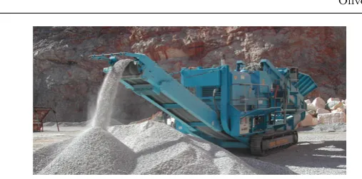
Fig. 1: A Terex Pegson MaxTrak1000 cone crusher.

Fig. 2: An idealised cone crusher cross-section.

Fig. 3: The critical physical parameters of the crusher.

1 Introduction

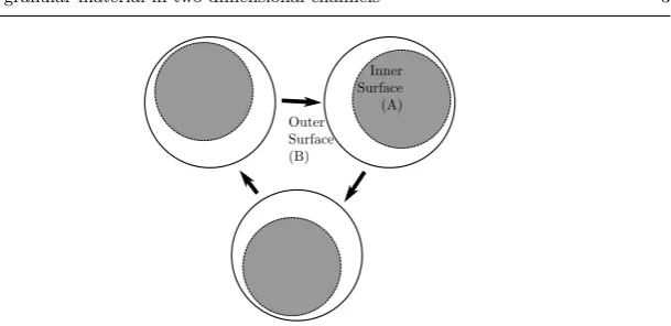
ap-Fig. 4: Illustration of the position of the inner mantle’s base at three time points, during its rotation about the concave’s axis of symmetry.

proximate two dimensional flows of pressure-crushable granular media within channel cross-sections similar to that shown in figure 3. Material to be crushed falls between the two surfaces, compacting locally where the inner mantle has greatest proximity to the concave. The mantle is fixed at its summit, while its base rotates on a circular path about the concave’s axis of symmetry, as in figure 4. We will consider the channel to have length L and height h at the inlet. The outlet heighthout at a given point on the circumference of the crusher will oscillate between minimum and maximum sizes at between four to ten cycles per second.

Within the literature the most prominent existing model for material flow and crushing within crushers was developed by Evertsson in his doctoral work [2, 3] from the earlier population model [4]. That approach was to establish a mass balance in combination with a flow and crushing model. The flow model is based on computing the path of each single particle through the crushing chamber, whether they be in freefall, sliding or crushing. The system is con-trolled by a ‘volumetric filling ratio’, ηv < 1, that allows for the incomplete filling in the inlet zone seen in real crushers. This model was then followed up by Evertsson and Lindqvist in collaboration with others [5–11] with the main intentions of improving the flow model and integrating lining wear into simulations. They optimized the geometry such that material experienced no sliding at the basal surface in its transit through the cross-section. In an in-dependent succeeding study [12–15], Evertsson’s results were refined further and successfully applied to an operational crusher and are now being incorpo-rated into new crusher design. The Evertsson model is interesting due to its discrete approach to the system, but the ultimate integral equation is a far less tractable model than our continuum fluid flow approximation, as we aim to examine the overall behaviour of the material and the quality of the output rather than to simulate the explicit grain trajectories and crushing.

- which equate roughly to gaseous, liquid and solid regimes - and generate the tractable, unifying models that still seem to be beyond our grasp. Much time has been put into modelling the gaseous phase using ‘granular temperatures’ [16], and the solid phase via solid mechanics [17], but the dense liquid flow has defied easy modelling. The dynamics/mechanics involved are complex, given the irregularly shaped particles which arise within any natural granular mate-rial, and random assemblies of these particles can lock together into temporary structures we refer to as force chains or networks [18–21]; which structures are sometimes also referred to as force eddies or clusters [22].

Instead of a discrete model, we choose to adopt a contiuum model that is minimal in nature and is based empirically on the study of the pseudo-liquid regime of flows of dense granular media, on an assumption of rock particles being small enough for a continuum approximation. The complexity and lack of consensus on modelling granular materials in the literature also make such an approximation credible in the context of our problem. Our chosen model is in essence composed of a pressure-dependent yield stress and an effective viscosity depending on the pressurep, grain diameterλand shear rate|γ˙|. In common with what we assume to occur inside the crushing cavity this material is pressure-thickening, which is analogous to the slowing and cessation of the fragments in the crusher as the crushing stroke occurs. Employing techniques used in computations involving Bingham viscoplastics [23] we choose to regu-larise the dimensional constitutive using the Bercovier-Engelman method. We can then apply the formerly piecewise and now universal constitutive relation over the whole channelΩ. The choice of regularisation is arbitrary in the sense that we could choose the Papanastasiou [24, 25] method equally well in the con-text of this work. With the prerequisite analysis we might invoke variational inequalities [26, 27] in place of regularisation, prompting a radically different formulation. We choose to invoke grain size dependence in this instance purely by its directly stated relation to the inertial numberI,

I=|γ˙|λ

ρs p

1/2

,

where deviatoric stressτ is given by

τ=µ(I) ˙γ,

and total stressσby

σ=−pI+τ ,

for close packed material densityρs, rate of strain tensor ˙γ, effective viscosity

functionµ(I), and identity tensorI.

In reality, many of the parameters, such as the coefficients ζs, ζ2, inertial constantI0, packing fractionκand Young’s ModulusEcmight also depend on

as stated, and neglect the influence of polydispersity in grain shape. Further

λ-dependence could be investigated in future work.

In the main body of this paper we will apply slip boundary conditions at both the physical boundaries. In the preliminary unidirectional work in section 2 we prescribe no-slip at the basal surface for a unique solution in the case of a parallel-sided channel. We prescribe basal slip in the ensuing two-dimensional work due to the assertions in [3], wherein it is stated clearly that there are three modes of movement for material within cone crushing machines: free fall from upper surface, ascendancy on the basal surface with the crushing concave and sliding on the basal surface. Evertsson states slip is common [3] but then optimises his model to avoid slippage. Within [28] it is again stated that slip is common within the first few layers of grains at the base.

We proceed by presenting a preliminary set of unidirectional solutions in section 2 which demonstrate our slip boundary condition and regularisation before moving on to the two-dimensional work. The variational formulation for the problem is given in section 3, the procedure for performing the calculations in section 4, some illustrative results are given in section 5 and a discussion is contained in section 6.

2 Preliminaries

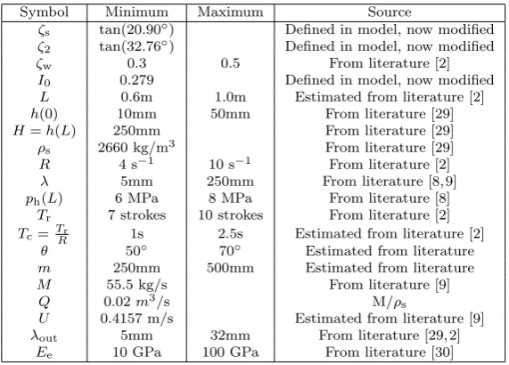
For ease of reference we list typical dimensional values for quantities involved in table 1. To begin, we examine the steady, non-inertial, gravity-driven and

Symbol Minimum Maximum Source

ζs tan(20.90◦) Defined in model, now modified

ζ2 tan(32.76◦) Defined in model, now modified

ζw 0.3 0.5 From literature [2]

I0 0.279 Defined in model, now modified

L 0.6m 1.0m Estimated from literature [2] h(0) 10mm 50mm From literature [29] H=h(L) 250mm From literature [29] ρs 2660 kg/m3 From literature [29]

R 4 s−1 _{10 s}−1 _{From literature [2]}

λ 5mm 250mm From literature [8, 9] ph(L) 6 MPa 8 MPa From literature [8]

Tr 7 strokes 10 strokes From literature [2]

Tc= T_Rr 1s 2.5s Estimated from literature [2]

θ 50◦ 70◦ Estimated from literature m 250mm 500mm Estimated from literature M 55.5 kg/s From literature [9] Q 0.02m3_{/s M/ρ}

s

U 0.4157 m/s Estimated from literature [9] λout 5mm 32mm From literature [29, 2]

Ee 10 GPa 100 GPa From literature [30]

Quantity Minimum Maximum Quantity Minimum Maximum ˆ

L 2 4 ˆh(0) 0.04 0.2 ˆ

h( ˆL) 1 Rˆ 0.64 1.6 ˆ

λ 0.02 1 pˆh 0.92 1.23

ˆ

Tc 6.26 15 Qˆ 0.204

ˆ

U 0.266 λˆout 0.02 0.128

ˆ

Ee 105 106

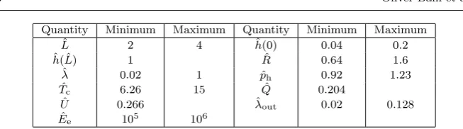
Table 2: Typical non-dimensional parameter values. See table 1 for dimensional version.

Fig. 5: The dimensional parallel-sided channel, inclined at angleθ to the hor-izontal.

incompressible flow of granular material in parallel-sided channels inclined at an angleθto the horizontal, as shown in figure 5.

From our table 2 of typical non-dimensional parameter values we can de-duce an approximate Froude numberFnof the form

Fn= U

2

gh =

0.41572

9.8×0.25 ≈0.07,

which number can stand in as an estimate for the Reynolds number in this case due to the pressure-dependence of the viscous stresses. SinceFn≈10−1,

we can consider the flow to be broadly non-inertial. Unidirectionality dictates that

u= (u(y),0),

τ =

0 τxy(y)

τyx(y) 0

andpsimplify to functions only ofy, the distance from the channel base. We non-dimensionalise the system using the scalings√ghfor velocity u, ρghfor stress-like quantitiesτ , p, Ee,hfor coordinatesx= (x, y) and grain diameterλ,

p

h/gfor timest andTc, and p

gh5_{for volumetric fluxQ.ρdenotes material}

density andgdenotes gravitational acceleration. Typical non-dimensional val-ues are shown in table 2. In line with this, the effective viscosityµ[1] simplifies to the following regularised

µreg du dy

, p, λ

=_q ζsp |du

dy|

2₊2

+ pλ √

κ(ζ2−ζs)

√

pI0+|du dy|λ

√

κ, (2)

and unregularised forms

µun du dy

, p, λ

= ζsp |du dy| + pλ √

κ(ζ2−ζs) √

pI0+|dudy|λ √

κ, (3)

whereis a small non-negative regularising parameter applied in the Bercovier-Engelman fashion [23], and the deviatoric stress is then defined by

τ =µ

du dy

, p, λ

˙

γ.

Our aim in preliminary studies is to find solutions of the unregularised and regularised JFP materials which may then be used to illustrate and validate our choices of slip condition and regularisation. These solutions may also be used as initial conditions for the two-dimensional calculations if necessary.

As in most fluid problems we will solve the system of equations formed by the equations of conservation of mass and momentum. Under our unidirec-tional assumption conservation of mass is described by

∇ ·u=∂u

∂x + ∂v ∂y,

and is automatically satisfied while conservation of momentum simplifies to

0 =Fx−∂p

∂x+ ∂τxx

∂x + ∂τyx

∂y =Fx+ dτyx

dy , (4a)

0 =Fy− ∂p ∂y+

∂τxy ∂x +

∂τyy

∂y =Fy− dp

dy, (4b)

whereF = (Fx.Fy) is the vector of gravity forces. We prescribe the boundary conditions

and employ the specific slip relation from [31], wherein tangential deviatoric stressτ_nt and velocityu_tvectors are defined at the wall by

u_t=u−(u·n)n,

τ_nt=τ·n−τnnn,

τnn = (τ·n)·n,

andnandtdenote normal and tangential vectors to the boundary, respectively. We prescribe the boundary stresses as both velocity- and pressure-dependent via

τ_nt=τ_slip(u_t, p) = τω

uω

u_t−_p ζwp

u2

ω+|ut|2

u_t. (5)

The quantity ζw is the material friction coefficient. ζs, ζw, and ζ2 can be alternatively understood via their relations to friction anglesφs, φw,φ2,

ζs= tanφs, ζ2= tanφ2, ζ2= tanφ2.

The quantities τω and uω are our boundary condition smoothing constants and represent small non-negative stresses and speeds, respectively, such that the approximation collapses down to the piecewise slip condition

(τ·n)·t=

(

ζwp if|u|>0,

numerical solution otherwise

as

uω→0,

τω

uω →0.

We in effect prescribe that for a material to slip at the boundary it must reach a threshold shear stressτslip∝p, hence making slip less likely for higher

ap-plied crushing pressureph. The term uτωωut exists as a guarantee of a bijective relation between slip stress and slip speed. Within the preliminary work it is simply implemented, while in the two-dimensional finite element calculations it is prescribed as a natural boundary condition, which requires the addition of complementary zero-flux terms in the variational formulation. For other ex-amples of slip boundary conditions and discussion see [28, 31, 32], while for a variational inequality possibility as applied to the Signorini boundary condi-tion problem see [33]. In this instance we choose regularisacondi-tion in line with our previous choice in the effective viscosity functionµ(I). Under unidirectionality, our prescribed slip stressτslip(5), simplifies to the scalar

τslip=− τω

uω

uh− ζwp

p

u2

−6 −5 −4 −3

_u

ω

10-5 10-4 10-3 10-2 10-1 100

||

u

ple

−

u

oth

|| ph

log10(τω/uω) =−5

log10(τω/uω) =−4

log10(τω/uω) =−3

log10(τω/uω) =−2

log10(τω/uω) =−1

log10(τω/uω) =0

Fig. 6: Convergence plots foruh for various configurations of (uω, τω). In this caseθ= 55◦,φs= 14◦,φw= 60◦,φ2= 75◦, and forph∈[0.01,1.5].

−6 −5 −4 −3

_u

ω

10-6 10-5 10-4 10-3 10-2 10-1 100

||

τ

ple

−

τ

oth

|| ph

log10(τω/uω) =−5

log10(τω/uω) =−4

log10(τω/uω) =−3

log10(τω/uω) =−2

log10(τω/uω) =−1

log10(τω/uω) =0

Fig. 8: Expected unidirectional flow in the parallel-sided channel, non-dimensional.

which in the piecewise case would dictate

τ(1) =−Fx(1−y0)

=ζwph,

y0 = 1 +ζwph

Fx ,

whereuh=u(h) is the slip speed. As a verification of our smoothed boundary condition we have run a sequence of calculations, and display the results in figures 6 and 7. We do indeed see that the smoothed boundary condition converges to the piecewise condition with decreasing uω and _uτω

ω in both the speed and stress fields.

We will solve the unregularised JFP system analytically with the exception of one key parametery0which must be found numerically in the event of non-slippage, while the regularised JFP system will be solved numerically using finite difference techniques.

2.1 The unregularised JFP system

Given the unregularised viscosity relation (3), the expression for the only non-zero deviatoric stressτyx=τxy under unidirectionality simplifies to

τyx=µun

du dy

, p, λ

du

dy =s ζsp+

du dy

pλ√κ(ζ2−ζs) √

pI0+|du dy|λ

√

κ

!

, (6)

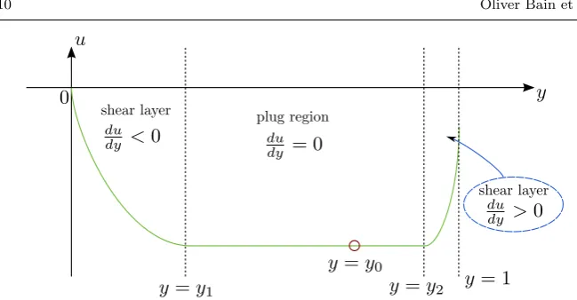
condition on the stress at the surface y = 1. The number of regions present is not constant and depends primarily on the applied normal stress ph. For the special case of a free surface situation when ph = 0, we anticipate that the material flow will consist of a single shear layer, but for all ph > 0 an unyielded region should exist. Generally, we expect the following three modes of behaviour to occur as we varyph:

– Free surface flow for zeroph, one shear layer,

– Slip for intermediateph, a plugged region and one or two shear layers,

– No-slip for largeph, a plugged region and two shear layers. Following from (4a) and (4b) we see

p=ph+Fy(y−h), (7a)

τyx=−Fx(y−y0). (7b)

Combining (7b) and (6) gives

τyx(y) =−Fx(y−y0) =ps ζs+

λ√κ|du

dy|(ζ2−ζs)

I0√p+λ√κ|du dy|

!

,

and rearranging yields

du dy =−

sI0

√

p

λ√κ

_τ−sζ

sp τ−sζ2p

, (8)

where

s= sgn

du dy

.

We solve equation (8) with the boundary conditions

u(0) = 0,

u(y2) =u(y1).

To integrate we use the substitution

t(y)2=p(y) =ph+Fy(y−1), (9a)

dy= 2t

Fydt, (9b)

where, under this substitution,

τ(y) =−Fx

Fy

t(y)2−t(y0)2

,

du dy =−

sI0√p λ√κ

_F

x+sζsFy Fx+sζ2Fy

t(y)

_t(y)2_−A s t(y)2_−A2

,

u(y) =− 2I0s

Fyλ√κ

_F

x+sζsFy Fx+sζ2Fy

Z

t(y)2

_t(y)2_−A s t(y)2_−A2

The equation foru(y) may be simplified as follows

u(y) =− 2sI0

Fyλ√κ

Fx+sζsFy Fx+sζ2Fy

Z

t(y)2+ (A2−As) +A2(A2−As)

t(y)2_−A2 dt,

where

As= Fxt(y0)

2

Fx+sζsFy ,

A2= Fxt(y0)

2

Fx+sζ2Fy.

We then integrate for the general solution

u(y) =− 2sI0

Fyλ√κ

Fx+sζsFy Fx+sζ2Fy

t(y)3

3 + (A2−As)t(y)

−pA2(A2−As) tanh−1

_t(y) √

A2

+ constant,

and apply our boundary conditions to find a piecewise solution. For 0≤y≤y1, we have

u(y) = 2I0

Fyλ

√

κ

_Fx−ζsFy

Fx−ζ2Fy

1 3(p(y)

3/2_−p(0)3/2₎

+(A2−As)(p(y)−p(y2))

−pA2(A2−As)

"

tanh−1

p

p(y) √

A2

!

−tanh−1

p p(0) √ A2 !#) ,

while fory1< y < y2 we find

u(y) =u(y1),

and finally foryy≤y≤1 we have

u(y) =u(y1)− 2I0

Fyλ√κ

_F

x+ζsFy Fx+ζ2Fy

1 3(p(y)

3/2_−p(y2)3/2₎

+(A2−As)(p(y)−p(y2))

−pA2(A2−As)

"

tanh−1

p

p(y) √

A2

!

−tanh−1

p

p(y2) √

A2

!#)

.

To determine the plugged region boundaries y1,y2, as shown in figure 8, we solve du_dy = 0, from equation (8):

0 = du

dy =τ−sζsp,

y= Fxy0−sζs(ph−Fy)

Fx+sζsFy ,

y1= Fxy0+ζs(ph−Fy)

Fx−ζsFy

, (15a)

y2= Fxy0−ζs(ph−Fy)

Fx+ζsFy

. (15b)

The boundary conditions onu(y) ensure continuity of the solution at y1, y2. The shear stress at the surfaceτhis determined indirectly by the chosen value ofy0. To find a solution consistent with the stress boundary condition we must numerically find a root iny0of the function

b(uh(y0)) =shph

"

ζs+| duh

dy |(ζ2−ζs)

p1_h/2+|duh

dy | #

− "

−τ ω

uω

uh−_pζwph

u2

ω+u2h uh

#

.

The surface velocityuhis determined by modifying the normal applied stress

phor the friction coefficientζw, but this may not be done arbitrarily as there are bounds on these two quantities which we shall now derive. Under uni-directionality the stress-strain relation for an unregularised JFP material, as detailed in [1], is given by

τ(y) =µ(I)p(y)s,

for

µ(I) =ζs+

I(ζ2−ζs)

I0+I

, (16a) I= du dy

λκ P

1/2

,

and therefore

µ(I) =sτ p.

Since, by the formulation of the constitutive relation in [1], we must have

ζs≤µ(I)≤ζ2,

it follows that at the base

−ζs(ph−Fy)

Fx ≤y0≤ −

ζ2(ph−Fy)

and then at the upper surface

1 +ζ2ph

Fx ≤y0≤1 + ζsph

Fx .

We combine the two inequalities on the assumption that there is an overlap in the regions fory0, and hence

−ζs(ph−Fy)

Fx

<1 +ζsph

Fx ,

−ζ2(ph−Fy)

Fx

>1 +ζ2ph

Fx ,

and gain the final requirement forph:

1 2ζ2

(ζ2Fy−Fx)< ph< 1

2ζs

(ζsFy−Fx). (18)

The bound on ph can be physically understood as the limiting pressure for

material flow. Above this limit the material is locked into a static arrangement due to its interlocking grains. The left hand side of (18) is uniformly negative forθ∈(φs, φ2) and so practically we have

max

0, 1

2ζ2

(ζ2Fy−Fx)

< ph< 1

2ζs

(ζsFy−Fx), (19)

since non-negative (pulling) applied normal stresses are non-physical in this case.

Further conditions on parameter ranges can now be determined based on the physical situations we wish to model and practicalities. For free surface flows we will needph= 0 and therefore a negative lower bound

1

2ζ2(ζ2Fy−Fx)<0,

ζ2> Fx

Fy = tanθ.

In the more general case of flows whereph>0 we look for other constraints;

we require a positive upper bound onph,

1

2ζs(ζsFy−Fx)>0,

tanθ= Fx

Fy > ζs.

Steady flow is therefore considered realistic for the JFP model under a bounded applied normal stressph if

0.0 0.2 0.4 0.6 0.8 1.0

y

−2.5 −2.0 −1.5 −1.0 −0.5 0.0

u

ph=0.01

ph=0.05

ph=0.10

ph=0.15

ph=0.20

ph=0.25

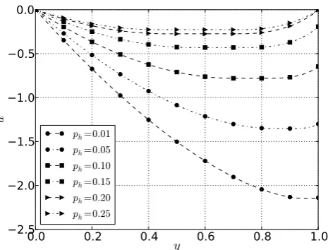
Fig. 9: Example plots of u(y) for various ph, plotted against y. In this case

θ= 55◦,ζs= tan 14◦,ζw= tan 60◦,ζ2= tan 75◦.

while no flow is possible for tan(θ)< ζsfor whateverph, and there speculatively could be unsteady flow for tan(θ)> ζ2for some values ofph. In light of these bounds on applied stress ph (19), and channel inclination θ (20), we modify the original values of ζs,ζ2. For sufficiently largeph we require smallζs, and

for largeθ we require largeζ2.

Limits for the the slip coefficient ζw are also built into the model. Since the edges of the unyielded ‘plug’ region are given by equations 15a, 15b we can deduce that for existence of a second shear layer and hence ‘controlled slippage’ we require

y2 <1,

ζw> ζs.

The ratioζw/ζsis, in addition toph, vital for the onset of slippage asζw/ζs>>

1. We may also speculate a similar change in behaviour with the ratioζw/ζ2

where slip decreases asζw/ζ2→1 for givenph.

−4 −3 −2 −1 0 1 2 3

du/dy

−0.8 −0.6 −0.4 −0.2 0.0 0.2 0.4

τ

ph=0.01

ph=0.05

ph=0.10

ph=0.15

ph=0.20

ph=0.25

Fig. 10: Example plots ofτ(y) for variousph, plotted against velocity gradient du

dy. In this caseθ= 55

◦_{,ζs= tan 14}◦_{,ζw= tan 60}◦_{,ζ2= tan 75}◦_.

Fig. 11: Discretisation of non-dimensionalu, τ overy∈[0,1].

2.2 The regularised JFP system

We regularise the JFP constitutive relation and introduce a parameter >0 such that the effective viscosity is given by (2). With the inclusion ofwe no longer have a tractable analytical problem and resort to numerical solution via finite difference techniques. We discretizeu,τandpoveryas in figure 11, and approximate the governing equations

0 =Fx+ dτyx

dy , du

dy =− sI0 λ√κ

√

p

_τ−sζsp

τ−sζ2p

when|τyx|> ζsp,

and boundary conditions

u(0) = 0,

τyx(1) =τslip=− τω

uω

uh− ζwp

p

u2

0.0 0.2 0.4 0.6 0.8 1.0

y

−0.35 −0.30 −0.25 −0.20 −0.15 −0.10 −0.05 0.00 0.05

u

log10(ǫ) =−3

log10(ǫ) =−2

log10(ǫ) =−1

log10(ǫ) =0

Fig. 12: Example plots ofu(y) for various, plotted against velocity gradient du

dy. Here we have θ = 55

◦_{, ζs = tan 14}◦_{, ζw = tan 60}◦_{, ζ2 = tan 75}◦_{, and}

ph= 0.25.

by the following system of 2n−1 equations

0 =Fx+τi−τi−1

∆y fori= 2, . . . , n−1, ui−ui−1

dy =− si−1I0

λ√κ pi−1

τi−1−sζspi−1 τi−1−si−1ζ2pi−1

fori= 2, . . . , n,

u0= 0,

τn−1=− τω

uω

un−_pζwpn−1

u2

ω+u2n un.

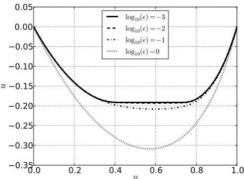
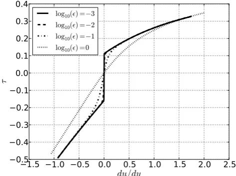
This is then solved using Newton’s method. We demonstrate convergence of the regularised solution to the unregularised with decreasing in figures 12 and 13. The regularisation effect is to increasingly eliminate the plugged re-gion in the velocity profile that we see in the unregularised profiles in figure 9. The regularisation is especially apparent in the stress profile where the discon-tinuity is clearly smeared, illustrating how over-regularisation fundamentally distorts the nature of the solutions computed. The regularisation parameter

−1.5 −1.0 −0.5 0.0 0.5 1.0 1.5 2.0 2.5

du/dy

−0.5 −0.4 −0.3 −0.2 −0.1 0.0 0.1 0.2 0.3 0.4

τ

log10(ǫ) =−3

log10(ǫ) =−2

log10(ǫ) =−1

log10(ǫ) =0

Fig. 13: Example plots ofτ(y) for various, plotted against velocity gradient du

dy. Here we have θ = 55

◦_{, ζs = tan 14}◦_{, ζw = tan 60}◦_{, ζ2 = tan 75}◦_{, and}

ph= 0.25.

3 Formulation

3.1 System

We now move on to examining flows of two-dimensional granular materials within non-parallel-sided channels, such as that shown in figure 14. The

ometry functionh(x) is given by

h(x) =hout+xtan(α) +x2

_3(h−hout)

L2 −

(2 tan(α) + tan(β))

L

+x3

_2(hout−h)

L3 +

tan(α) + tan(β)

L2

, (22)

which has been designed to satisfy conditions

h(0) =hout, h(L) = 1, h0(0) = tan(α), h0(L) = tan(β).

We retain our previous scalings and our non-inertial and incompressible flow assumptions. The whole time-dependent problem is modelled as a sequence of quasi-steady fluid problems. Since this viscoplastic constitutive relation was designed for generic granular materials, we modify some of the model param-eters for quantitative similarity to our real life crusher.

The crusher cross-section is approximated as a two-dimensional channel of fixed geometry. The fixed geometry is chosen since the moving boundary problem would be problematic in combination with our assumption of incom-pressibility, while the crushing stroke is simulated by a prescribed applied stressph(t) at the inlet. This idealised cross-section is a minimal model that represents approximately the effective crushing portion of the cross-section. The pressure drop from inlet to outlet is a necessary compromise to drive the fluid continuum approximation to the granular material, in addition to the gravity forces which will cause flow under sufficiently small applied normal stress.

We will solve a sequence of quasistatic problems in velocity u(x;t) and pressure p(x;t) for fixedλin space, linked by a constitutive problem in time and space for λ and fixed u, p. Assuming small enough time steps we can assemble the solutions to these two problems into a larger composite solution for (u, p, λ).

Following, the two dimensional viscoplastic fluid problem in velocity u= (u, v) and isotropic pressurepis composed of the equations of conservation of mass and momentum as follows

0 =∇ ·u, (23a)

0 =F+∇ ·σ, (23b)

which are equivalent to the following in terms ofu= (u, v) andp,

0 =∇ ·u,

0 =F− ∇p+∇ · {φγ˙},

where we have the regularised non-dimensional constitutive relation defining the effective viscosity φas non-linearly dependent on ˙γ, pand particle sizeλ

by

φ(|γ˙|, p) =

_ζs

(2_+|γ˙|2₎1/2+

λκ1/2(ζ2−ζs)

I0p1/2+λκ1/2|γ˙|

The volume fraction κ is assumed constant in line with our assumption of incompressibility. This system is accompanied by the following boundary con-ditions

u·n= 0 aty=h(x) andy= 0,

(τ·n)·t=τslip(u) aty=h(x) andy= 0,

p=pin(y) at the inlet (x=L), p=pout(y) at the outlet (x= 0), v= 0 at the outlet and inlet, σ·n=pin(y)n at the inlet,

σ·n=pout(y)n at the outlet,

where the pressurephas been carefully prescribed at the inlet and outlet due to the pressure-dependence in the constitutive relation. The pressure conditions at the inlet and outlet are completed by

pin(y) =ph(t) +Fy(y−1), (25a)

pout(y) =ph(t)−pstep+Fy(y−1)hout, (25b)

ph(t) =ph,low+ (ph,high−ph,low)

h

1 + sin2πRt−π 2

i

, (25c)

which describe oscillatory applied stresses at those boundaries with a finite pressure drop pstep from inlet to outlet, bounds at the inlet for the applied stress ofph,lowandph,high, and crushing stroke frequencyR.

The partial differential equation for the particle sizeλis given by

Dλ Dt =−

λδ

4Tc

(1 + tanh(Υ(p−pcrush)))(1−tanh(ψ(x−xcrush))), (26)

where

λ=houtatt= 0, λ=houtatx=L.

This represents an approximation to a simple crushing switch such that rock fragments reduce in size given pressure larger than the thresholdpcrush, which is given below, and a lack of proximity to the inlet, where xcrush defines the transition from the inlet zone to the crushing zone. Here, δ is our control parameter to adjust the rate of crushing, Tc is a represenative travel time through the crusher, and we take results from [35–38] in our derivation of the

λ-dependentpcrush given by

pcrush=cEe π

sc

λ

2

!3/2

=cEe π

_2sc

λ

3/2

. (27)

We have assumed rough symmetry in the grains in defining pcrush, and little

plasticity for the contact displacementsc and point out that the constantcis

the modifier found in [37], to be commonly in the range

0.2< c <0.3.

– A pressure-thickening material,

– Effective pressure-roughening at the boundaries,

– Pressure-dependent crushing.

3.2 Variational form

We now derive variational forms for use in the finite element approximation of the underlying system of partial differential equations. We define ¨u, ¨v, ¨p, ¨λas test functions associated with our unknowns. Concentrating first on our fluid problem we multiply equation (23a) by ¨pand (23b) by (¨u,v¨), integrate over the channelΩ, and then apply integration by parts to obtain

0 =

Z

Ω ¨

p∇ ·u dx, (28a)

0 =

Z

Ω ¨

u·F−σ· ∇·u dx¨ +

Z

∂Ω

n·σ·u ds.¨ (28b)

We use the surface integrals to prescribe our natural boundary conditions onτ

andp, but must enforce zero flux across the physical boundaries via additional terms [39] in the variational formulation:

+

Z

∂Ωslip

¨

pn·u ds,

− Z

∂Ωslip

ξ(u·n)(¨u·n)ds,

whereξis given by

ξ≈ 10q

2

he .

The new quantityqis the polynomial degree of ¨uand ¨v, whileheis a piecewise constant function defined overΩ, which indicates the diameter of each element in the mesh. We choose approximating functions of the form

u, v piecewise bilinears plus cubic bubbles,

p, λ piecewise bilinears,

and selectq= 2 as a compromise between the linear and cubic portions of our approximating functions and as a value in line with the ideal but computa-tionally expensive biquadratic functions normally used to satisfy the stability condition. The variational forms for the fluid problem upon rewriting in terms ofτ andpare therefore

0 =

Z

Ω ¨

p∇ ·u dx− Z

∂Ωslip

¨

0 =

Z

Ω ¨

u·F−(σ· ∇)·u dx¨ +

Z

∂Ωin

−(n·¨u)pin+Λ(τ·n)·u ds¨

+

Z

∂Ωslip

(n·u¨)(−p+ [τ·n]·n) + (t·u¨)τslip(t·u, p)ds

− Z

∂Ωslip

ξ(u·n)(¨u·n)ds+

Z

∂Ωout

−(n·¨u)pout+Λ(τ·n)·¨u ds,

where Λ ∈ [0,1] is a continuation parameter which we reduce during the calculation to achieve our normal stress boundary conditions at the inlet and outlet.

Moving on to the particle size problem, we discretize equation (26) in time, by effectively approximating

∂λ ∂t ≈

λt−λold ∆t ,

for small time step∆t. We therefore obtain

Dλ Dt ≈

λ−λold

∆t + (u· ∇)λ

=−δλ 4Tc

(1 + tanh(Υ(p−pcrush)))·(1−tanh(ψ(x−xcrush))), (31)

Particle sizeλis paired with its test function ¨λfrom a piecewise bilinear finite element space and the system integrated over the channelΩ, to arrive at

T(λ,¨λ) =

Z

Ω ¨

λ

_λ

−λold

∆t + (u· ∇)λ

+ δ ¨

λλ

4Tc(1 + tanh(Υ(p−pcrush)))·(1−tanh(ψ(x−xcrush)))dx

= 0. (32)

We retain the initial and boundary conditions already stated.

4 Procedure

We compute our numerical solutions using Newton’s method, and explicit time-stepping for theλ-problem. We employ sufficiently small time steps, de-duced from typical values in table 2, such that we will not have problems with the Courant Friedrichs Lewy (CFL) condition. Specifically we make an estimate such that material should not travel more than an average element diameter ¯he in distance over a time step∆t.

We adopt the procedure illustrated in figure 15, noting that the initial continuation from the parallel-sided to non-parallel sided channel problem includes continuation on five parameters simultaneously in a vectorG:

Fig. 15: General procedure for solving the time-dependent sequence of prob-lems.

5 Results

We define the following functionals

M(χ) =

R Aχ dx

AA ,

ς(χ) =

Z

A

(χ−M(χ))2dx

1/2

,

M2(χ) = 1

t2−t1

Z t2

t1

χ dt,

where M represents a spatial mean, ς is the ‘consistency’ and is equivalent to a standard deviation, andM2 is a temporal mean. ‘Improved’ consistency

refers to a smaller value forς.

In solving our system of equations we have prescribed a fixed time step

∆t and set the model constants (I0, ζs, ζ2, c, δ) such that the results are of

the correct order of magnitude upon settling to their regular patterns. Those reference constants are shown in table 3, and our solution exhibits

M(|u|) = 0.327, M(λout) = 0.011,

which is satisfactorily similar to the typical reference nondimensionalised val-ues shown in table 2. We establish a set of reference points down the channel,

θ = 65◦ _φ

s = 8◦ φw = 25◦

φ2 = 75◦ ph,low = 0.7 ph,high = 1.2

log10() = 0 I0 = 10 pstep = 0.4

log10(τω) = −4 log10(uω) = −1 κ = 0.7

sc = 0.0001 c = 0.0278 Ee = 100000

δ = 4.5 R = 1 Tc = 7

log10(Υ) = 1 log10(ψ) = −0.2

Table 3: Parameter set for the reference problem, with associated figures 17-22.

Fig. 16: Reference points along mid-line of channel. x_i = iL

6, 1 2h

iL

6

, for

66 68 70 72 74

t

10-2 10-1 100

λ

x0 x1 x2 x3 x4 x5 x6

Fig. 17:λat the reference points shown in figure 16.

66 68 70 72 74

t

0.0 0.2 0.4 0.6 0.8 1.0 1.2 1.4 1.6

ph Q M(|u|)

Fig. 18:ph, QandM(|u|).

so-66 68 70 72 74

t

−0.8 −0.6 −0.4 −0.2 0.0 0.2 0.4 0.6

M(|u|) ς(|u|) Ref U

Fig. 19:M(|u|) andς(|u|).

66 68 70 72 74

t

100

p

x0 x1 x2 x3 x4 x5 x6

Fig. 20:pat the reference points shown in figure 16.

66 68 70 72 74

t

10-7 10-6 10-5 10-4

pin test pout test Flux

Fig. 21:pin,pout and flux measures.

66 68 70 72 74

t

10-2 10-1 100 101

ph Slip high Slip base

Fig. 22: Slip measures aty= 0 andy=h(x).

10-1 100 ₁₀1 ω

10-5 10-4 10-3 10-2 10-1

M2(M(λout)) M2(ς(λout)) M2(M(|u|)) M2(ς(|u|))

Fig. 23: Plots of M2(M(λout)), M2(ς(λout)), M2(M(|u|)), M2(ς|u|) for R = 0.25,0.5,1.0,2.0,4.0, where we have computedM2averages overt∈[59,75].

5.1 Varying stroke frequency

In our reference solution we have a typical non-dimensionalised crushing stroke frequency R = 1. We follow the tuning procedure with a set of calculations for R = [0.25,0.50,1.00,2.00,4.00] over time t ∈ [50,75], where we employ continuation on R at t= 50. We then calculate our measures M2(M(λout)),

M2(ς(λout)), |M2(M(|u|))|, M2(ς|u|) over t ∈ [59,75] and plot in figure 23.

In three of the four measures we see no discernible variation over R, while a slight deteriation in output consistency can be seen with increasingR. This is worthy of further consideration, and would be of great interest in the full three dimensional model.

5.2 Varying stroke strength

We now investigate the effect of altered crushing stroke strength on the output quality and quantity. We employ continuation att= 50 and calculate solutions forph,high= 1.0,1.1,1.2,1.3,1.4. The bottom line results are plotted in figure

24 and seem to illustrate that increasing the crushing strength both reduces the average grain size of the output but also the average speed of the material. The consistency measures both reduce with increasingph,high, reflecting more

10-1 100 ₁₀1 ph

10-5 10-4 10-3 10-2 10-1

M2(M(λout)) M2(ς(λout)) M2(M(|u|)) M2(ς(|u|))

Fig. 24: Plots of M2(M(λout)), M2(ς(λout)), M2(M(|u|)), M2(ς|u|) for

ph,high = 1.0,1.1,1.2,1.3,1.4, where we have computed M2 averages over t∈[59,75].

6 Discussion

In this article we have formulated a two-dimensional system and its varia-tional equivalent, which approximates the flow of granular material in a two-dimensional fixed geometry cone crusher cross-section. By manipulating the model parameters as set out for the viscoplastic constitutive law and adding a simple crushing rule we can approximate the flow of granular material and crushing under compressive crushing pressure in the channel. The crushing stroke in the fixed two-dimensional geometry is simulated by an oscillatory applied normal stress at the inlet and outlet, which can be modified in both frequency and size to assess the influence of those factors on the output size and consistency.

From our initial investigations it seems that adjusting the frequency of the crushing stroke has very little effect on the quality or quantity of the output. There is a somewhat surprising result of improved consistency of output for small frequencies which should be investigated further, which is potentially linked to the fact that for such small frequencies the stroke period approaches that of the transit time of the material in the crusher. Predictably increasing the crushing strength does reduce the mean output size and improve the con-sistency of the output. This greater degree of crushing is offset by a reduced throughput of material.

ap-proximation to the real-life crusher situation we need to investigate methods for facilitating such flows of granular media without the pressure difference. Increasing the inertial referenceI0can suffice to a certain extent but saturates quickly. Reductions in the friction coefficient ζw can also boost throughput but very small ζw and ph can cause computational problems due to infinite

slippage and a model that requires non-negative pressure. The pressure ‘hump’ that exists mid-channel will also retard flow via the slip boundary conditions at the top and base as well as thickening the medium. The pressure satisfac-tion tests show errors on the order of 10−6 _{at the inlet and outlet, which are}

to be considered satisfactory. A further simplification has been in the minimal choice of particle size dependence via the Inertial NumberI, which should be re-evaluated in future research. Overall, this work provides a promising foun-dation for future work while being a ground-breaking first attempt to model the flow in a rock crusher using a rational, continuum approach.

Future work will be devoted to the three-dimensional generalisation of this problem, beginning with the fixed geometry problem and moving on to the moving boundary version.

Acknowledgements We would like to thank the EPSRC and Terex Pegson, especially Ian Boast and Tim Cummings of Terex Pegson, for their promotion and sponsorship of this CASE project. We also thank the the University of Nottingham for their wonderful staff and facilities.

References

1. Pierre Jop, Yo¨el Forterre, and Olivier Pouliquen. A consitutive law for dense granular flows. Nature, 441:727–730, 2006.

2. C.M. Evertsson. Modelling of flow in cone crushers. Minerals Engineering, 12(12):1479– 1499, 1999.

3. C.M. Evertsson. Cone crusher performance. PhD thesis, Department of Machine and Vehicle Design, Chalmers University of Technology, Sweden, 2000.

4. SR Broadbent and TG Callcott. A new analysis of coal breakage processes. Journal of the Institute of Fuel, 29:524–539, 1956.

5. M. Lindqvist and C.M. Evertsson. Prediction of worn geometry in cone crushers. Minerals Engineering, 16(12):1355–1361, December 2003.

6. M. Lindqvist and C.M. Evertsson. Improved flow- and pressure model for cone crushers. Minerals Engineering, 17(11-12):1217–1225, 2004.

7. Magnus Bengtsson and C. Magnus Evertsson. An empirical model for predicting flaki-ness in cone crushers. Journal of Mineral Processing, 79:49–60, 2006.

8. M. Lindqvist and C.M. Evertsson. Development of wear model for cone crushers. Wear, 261:435–442, 2006.

9. Mats Lindqvist, Magnus Evertsson, Tapiwa Chenje, and Peter Radziszewski. Influence of particle size on wear rate in compressive crushing. Minerals Engineering, 19:1328– 1335, 2006.

10. Erik Hulth´en and C. Magnus Evertsson. Algorithm for dynamics cone crusher control. Minerals Engineering, 22:296–303, 2009.

11. E Lee and C.M. Evertsson. A comparative study between cone crushers and theoretically optimal crushing sequences (in press). Minerals Engineering, 2010.

13. Huang Dongming, Fan Xiumin, Wu Dianliang, and Fusheng Yao. Research on cone crusher chamber geometry. China Mechanical Engineering, 19(17):2041–2045,2049, 2008.

14. Dong Gang, Fan Xiumin, and Huang Dongming. Analysis and optimization of cone crusher performance. Minerals Engineering, 2009.

15. Dong Gang, Huang Dongming, and Fan Xiumin. Cone crusher chamber optimization using multiple constraints. International Journal of Mineral Processing, 93:204–208, 2009.

16. Isaac Goldhirsch. Rapid granular flows. Annual Review of Fluid Mechanics, 35:267–293, 2003.

17. R.M. Nedderman. Statics and Kinematics of Granular Materials. Cambridge University Press, 1992.

18. H.A. Janssen. Versuche ¨uber getreidedruck in silozellen. Zeitschr. d. Vereines deutscher Ingenieure, 39:1045, 1895.

19. Matthias Sperl. Experiments on corn pressure in silo cells - translation and comment of Janssen’s paper from 1895. Granular Matter, 8:59–65, 2006.

20. T. Boutreux, E. Rapha¨el, and P.G. de Gennes. Propagation of a pressure step in a granular material: The role of wall friction. Physical Review E, 55(5):5759–5773, May 1997.

21. P.G. de Gennes. Granular matter: A tentative view. Reviews of Modern Physics, 71(2):S374–S382, Centenary 1999.

22. D. Erta¸s and T.C. Halsey. Granular gravitational collapse and chute flow. Europhysics Letters, 60(6):931–937, 2002.

23. Edward J. Dean, Roland Glowinski, and Giovanna Guidoboni. On the numerical sim-ulation of Bingham visco-plastic flow: Old and new results. Journal of Non-Newtonian Fluid Mechanics, 142:36–62, 2007.

24. Tasos C. Papanastasiou. Flows of materials with yield. Journal of Rheology, 31(5):385– 404, 1987.

25. T.C. Papanastasiou and A.G. Boudouvis. Flows of viscoplastic materials: Models and computations. Computers and Structures, 64(1-4):677–694, 1997.

26. David Kinderlehrer. Variational inequalities and free boundary problems. Bulletin of the American Mathematical Society, 84(1):7–26, January 1978.

27. R.R. Huilgol. Variational inequalities in the flows of yield stress fluids including inertia: Theory and applications. Physics of Fluids, 14(3):1269–1283, March 2002.

28. Birte Domnik and Shiva P Pudasaini. Full two-dimensional rapid chute flows of simple viscoplastic granular materials with a pressure-dependent dynamic slip-velocity and their numerical solutions. Journal of Non-Newtonian Fluid Mechanics, 173-174:72–86, 2012.

29. R.A. Bearman and C.A. Briggs. The active use of crushers to control product require-ments. Minerals Engineering, 11(9):849–859, 1998.

30. John M. Ide. Comparison of statically and dynamically determined Young’s Modulus of rocks. Proceedings of the National Academy of Sciences, 22(2):81–92, 1936. 31. Nicolas Roquet and Pierre Saramito. An adaptive finite element method for viscoplastic

flows in a square pipe with stick-slip at the wall. Journal of Non-Newtonian Fluid Mechanics, 155:101–115, 2008.

32. I.J. Rao and K.R. Rajagopal. The effect of the slip boundary condition on the flow of fluids in a channel. Actu Mechanica, 135:113–126, 1999.

33. Gabriel N Gatica, Matthias Maischak, and Ernst P Stephan. Numerical of a transmission problem with Signorini contact using mixed-FEM and BEM. ESAIM: Mathematical Modelling And Numerical Analysis, 45:779–802, 2011.

34. Paulo R. de Souza Mendes, Mˆonica F. Naccache, and Priscilla R. Varges. Flow of viscoplastic liquids through axisymmetric expansions-contractions. Journal of Non-Newtonian Fluid Mechanics, 142(1-3):207–217, March 2007.

35. Ali Daouadji and Pierre-Yves Hicher. An enhanced constitutive model for crushable granular materials. International Journal for Numerical and Analytical Methods in Geomechanics, 34:555–580, 2009.

37. P.H. Shipway and I.M. Hutchings. Attrition of brittle spheres by fracture under com-pressionand impact loading. Powder Technology, 26:23–30, 1993.

38. Charlotte Couroyer, Zemin Ning, Mojtaba Ghadiri, Nathalie Brunard, Fr´ed´eric Kolenda, Denis Bortzmeyer, and Philippe Laval. Breakage of macroporous alumina beads un-der compressive loading: simulation and experimental validation. Powun-der Technology, 105:57–65, 1999.