The Thirty-Third AAAI Conference on Artificial Intelligence (AAAI-19)
Constraint-Based Sequential Pattern Mining with Decision Diagrams
∗Amin Hosseininasab,
1Willem-Jan van Hoeve,
1Andre A. Cire
21Tepper School of Business, Carnegie Mellon University, USA 2Dept. of Management, University of Toronto Scarborough, Canada
[email protected], [email protected], [email protected]
Abstract
Constraint-based sequential pattern mining aims at identify-ing frequent patterns on a sequential database of items while observing constraints defined over the item attributes. We in-troduce novel techniques for constraint-based sequential pat-tern mining that rely on a multi-valued decision diagram (MDD) representation of the database. Specifically, our repre-sentation can accommodate multiple item attributes and var-ious constraint types, including a number of non-monotone constraints. To evaluate the applicability of our approach, we develop an MDD-based prefix-projection algorithm and com-pare its performance against a typical generate-and-check variant, as well as a state-of-the-art constraint-based sequen-tial pattern mining algorithm. Results show that our approach is competitive with or superior to these other methods in terms of scalability and efficiency.
Introduction
Sequential Pattern Mining (SPM) is a fundamental data min-ing task with a large array of applications in marketmin-ing, health care, finance, and bioinformatics, to name a few. Fre-quent patterns are used, e.g., to extract knowledge from data within decision support tools, to develop novel association rules, and to design more effective recommender systems. We refer the reader to (Fournier-Viger et al. 2017) for a re-cent and thorough review of SPM and its applications.
In practice, mining the entire set of frequent patterns in a database is not of interest, as the resulting number of items is typically large and may provide no significant in-sight to the user. It is hence desirable to restrict the mining algorithm search to smaller subsets of patterns that satisfy problem-specific constraints. For example, in online retail click-stream analysis, we may seek frequent browsing pat-terns from sessions where users spend at least a minimum amount of time on certain items that have specific price ranges. Such constraints limit the output of SPM and are much more effective in knowledge discovery, as compared to an arbitrary large set of frequent click-streams.
A na¨ıve approach to impose constraints in SPM is to first collect all unconstrained frequent patterns, and then to apply
∗
This work was supported by ONR grant N00014-18-1-2129.
Copyright c⃝2019, Association for the Advancement of Artificial
Intelligence (www.aaai.org). All rights reserved.
a post-processing step to retain patterns that satisfy the de-sired constraints. This approach, however, may be expensive in terms of memory requirements and computational time, in particular when the resulting subset of constrained pat-terns is small in comparison to the full unconstrained set. Constraint-based sequential pattern mining (CSPM) aims at providing more efficient methods by embedding constraint reasoning within existing mining algorithms (Pei, Han, and Wang 2007; Negrevergne and Guns 2015). Nonetheless, while certain constraint types are relatively easy to incor-porate in a mining algorithm, others of practical use are still challenging to handle in a general and effective way. This is particularly the case of non-monotone constraints represent-ing, e.g., sums and averages of attributes.
Contributions.In this paper, we propose a novel represen-tation of sequential database using a multi-valued decision diagram (MDD), a graphical model that compactly encodes the sequence of items and their attributes by leveraging sym-metry. The MDD representation can be augmented with constraint-specific information, so that constraint satisfac-tion is either guaranteed or enforced during the mining algo-rithm. Finally, as a proof of concept, we implement a general prefix-projection algorithm equipped with an MDD to en-force several constraint types, including complex constraints such as average (“avg”) and median (“md”). To the best of our knowledge, this paper is the first to consider the “sum,” “avg,” and “md” constraints with arbitrary item-attribute as-sociation within the pattern mining algorithm. Lastly, we provide an experimental comparison on real-world bench-mark databases, and show that our approach is competitive with or superior to a state-of-the-art CSPM algorithm.
Related work
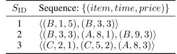
Table 1: ExampleSD, with attributes of time and price.
SID Sequence:{(item, time, price)}
1 ⟨(B,1,5),(B,3,3)⟩
2 ⟨(B,3,3),(A,8,1),(B,9,3)⟩
3 ⟨(C,2,1),(C,5,2),(A,8,3)⟩
where events have no specific order (Soulet and Cr´emilleux 2005; Bistarelli and Bonchi 2007; Bonchi and Lucchese 2007; Le Bras, Lenca, and Lallich 2009; Leung et al. 2012), as well as in CSPM when items and attributes are inter-changeable (Pei, Han, and Wang 2007).
Recently, constraint programming (CP) has emerged as a successful tool for CSPM (Negrevergne and Guns 2015; Kemmar et al. 2016; Kemmar et al. 2017; Aoga, Guns, and Schaus 2017; Guns et al. 2017). CP search techniques, albeit general, can potentially be more efficient when compared to specialized CSPM algorithms. Nonetheless, they still rely on constraint-specific properties to effectively prune unde-sired patterns.For example, (Aoga, Guns, and Schaus 2017) show how to effectively implement a number of prefix anti-monotone constraints into CP, but indicate that post-processing is still required to handle monotone constraints such as the minimum span.
Graphical representations of a database have been shown to be effective in item-set mining (Han et al. 2004; Pyun, Yun, and Ryu 2014; Borah and Nath 2018) and SPM (Masseglia, Poncelet, and Teisseire 2009). Previous works have also applied binary decision diagrams as a database modeling tool (Loekito and Bailey 2006; Loekito and Bailey 2007; Loekito, Bailey, and Pei 2010; Cambazard, Hadzic, and O’Sullivan 2010), which are effective when the se-quences of the database are similar, but typically do not scale otherwise. We show that our MDD representation retains its size regardless of the similarity between sequences, and pro-vides a more concise representation in the context of SPM.
Problem definition
We next formally describe the SPM problem and then dis-cuss the handling of constraints.
The SPM database and mining algorithm
The SPM database consists of a set of events, which are modeled by a set of literalsIdenoted byitems. Itemsi∈I
are associated with a set ofattributesA={A1, ...,A|A|
}
; for example, attributes can be price, quality, or time. A se-quence databaseSDis defined as a collection ofNitem se-quences{S1, S2, . . . , SN}, where all sequences are ordered
with respect to the same attributeA ∈ A; e.g., occurrence
in time. Table 1 illustrates an exampleSD withN := 3,
|I| := 3, andM := max
n∈{1,...,N}{|Sn|} = 3, where items
i∈Iare associated with time and price attributes.
The SPM task asks for the set of frequentpatternswithin
SD. A pattern P = ⟨i1, i2, . . . , i|P|⟩is a subsequence of
someS ∈ SD. LetS[j]denote thejthposition (i.e., item)
of sequenceS. A subsequence relationP ≼Sholds if and
only if there exists an embeddinge: e1 ≤e2 ≤... ≤e|P|
such that S[ej] = ij, ij ∈ P. For example, P = ⟨A, B⟩
is a subsequence of S = ⟨A, B, C, B⟩ with two possible embeddings(1,2)or(1,4). We define a super-sequence re-lation S ≽ P analogously, with “≤” replaced by “≥”. A pattern is frequent if it is a subsequence of at leastθnumber of sequences inSD, whereθis a given frequency threshold. The two best-known mining algorithms for SPM are the Apriori algorithm introduced by (Agrawal, Srikant, and oth-ers 1994), and the prefix-projection algorithm introduced by (Han et al. 2001). Both are iterative procedures and operate by extending frequent patterns one item at a time. In Apriori, candidate patterns are generated by expanding a pattern with all available items, and thereafter checking the frequency of generated candidates. As candidates may or may not be frequent, the Apriori algorithm suffers from the exponen-tial explosion of the number of generated candidates and redundancy. The prefix-projection algorithm, in turn, oper-ates by projecting each sequence S ∈ SD onto a small-est subsequenceS¯=⟨i1, i2, . . . , ij⟩, denoted byprefix, and
searching for frequent items in this reduced database. Any sequence that is obtained by extending a frequent prefix is guaranteed to be frequent in the original database. Prefix-projection is more efficient than the Apriori algorithm as it rules out infrequent patterns more effectively, but it requires the full database to be in memory (Han et al. 2001).
Constraint satisfaction in CSPM
A constraintCtype(·)is a Boolean function imposed on
ei-ther the patterns or their attributes. A pattern P satisfies a constraint if and only ifCtype(P) = true. The objective
of CSPM is to find all frequent patterns that satisfy a set of user-defined constraints. In particular, the challenge of CSPM is to impose constraints during the mining algorithm, rather than post-processing mined patterns for constraint sat-isfaction.
The standard framework for CSPM is to classify straints as being monotone or anti-monotone, as such con-straint are easy to handle within the mining algorithm (Pei, Han, and Wang 2007).1 A constraint ismonotoneif its
vio-lation by a sequenceSimplies that all subsequencesS¯≼S
also violate the constraint.
A constraint is anti-monotone if its violation by a se-quenceS implies violation by all super-sequencesSˆ ≽S. Table 2 lists common constraint types with their charac-terization. The concepts of monotonicity, anti-monotonicity, and violation are analogously extended to prefixes.
Constraints that are neither monotone nor anti-monotone are called non-monotone and are the most challenging to enforce during mining. While dedicated approaches have been developed for certain non-monotone constraints (Pei, Han, and Wang 2007), they are otherwise handled by post-processing (Aoga, Guns, and Schaus 2017). Our goal is to develop a generic platform to handle non-monotone con-straints effectively.
1
Table 2: Characterization of constraints as monotone (M), anti-monotone (AM), or non-monotone (NM) for SPM.
Name Constraint:=definition M AM NM
Maximal Cmxl(P) :=@P′∈ SD:P≺P′ •
Sup-Patt Cspt(P) :=∃P′∈ SD:P′≺P •
Length Clen(P)≥c:=|P| ≥c •
Clen(P)≤c •
Reg Expr Creg(P) :=P[i]∈I¯⊂I ⋆
Gap Cgap(A)≤c:=αj−αj−1≤c, ⋆
αj∈ A,2≤j≤ |P|
Cgap(A)≥c •
Span Cspn(A)≤c:= max{A} −min{A} ≤c •
Cspn(A)≥c •
Max/Min Cmax(A)≥c, Cmin(A)≤c • Cmax(A)≤c, Cmin(A)≥c •
Stats Csum(A), Cavg(A), Cvar(A), Cmed(A) •
⋆Not anti-monotone, but prefix anti-monotone.
An MDD representation for
SD
MDDs are widely applied as an efficient data structure in verification problems (Wegener 2000) and were more re-cently introduced as a tool for discrete optimization and con-straint programming (Bergman et al. 2016). Here, we use an MDD to fully encode the sequences fromSD; we refer to such data structure as anMDD database. We show how con-straint satisfaction is achieved by storing concon-straint-specific information at the MDD nodes, thereby removing the need to impose constraint-specific rules in a mining algorithm.
MDD construction for the SPM problem
An MDDM = (U, A)is a layered directed acyclic graph, whereUis the set of nodes, andAis the set of arcs. SetUis partitioned into layers(l0, l1, ..., lm+1), such that layersli :
1≤i≤mcorrespond to position (item)iof a sequenceS∈ SD. Layersl0, andlm+1consist of single nodes, namely the
root noder∈l0, and the terminal nodet ∈lm+1. The root
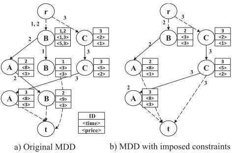
and terminal node are used to model the start and end of all sequences, respectively. Figure 1.a shows the MDD database model for theSDof Table 1.
Layerslj,1≤j ≤m, contain one node per itemi∈I :
∃S ∈ SD, S[j] =i, and model the possible items at posi-tionjof all sequencesS ∈ SD. For example, layer 1 of the MDD database in Figure 1.a has two nodes corresponding to itemsB, C, and no node associated to itemA. To distinguish which nodes are associated to which sequencesS∈ SD, we define labelsdufor nodesu∈ U, and store the associated
sequence indexSIDindu. The first label of nodeBat layer
1 of Figure 1.a, indicates that sequences 1 and 2 contain item
Bat their first position. In addition, we store the attribute la-bels associated with the item, one perSIDat each node. For
example, in Figure 1.a we store the time and price attributes. An arca = (u, v) ∈ A, is directed from a nodeu ∈ lj
to a nodev ∈lj′ : j′ > j, and represents the next possible
item after nodeu, for all sequences inSD. Similar to nodes
u∈U, labelsda are defined for arcsa∈Aand store their
associated sequences. A sequenceS is thus represented by a path fromrtot, following the nodes and arcs associated toSID. As we will search the MDD for patterns during the
B <1,3>1,2 <5,3> C
3 <2> <1>
A B C <5>3 <2>
A B
1 2
3
3 2
r
t
1, 2 3
ID <time> <price>
3 <8> <3>
1 <3> <3>
2 <9> <3>
B <3>2 <3> C
3 <2> <1>
A C <5>3
<2>
A 2
3
2 <8>
<1> 3
r
t
2 3
3 <8> <3>
2 3
2 <8> <1>
a) Original MDD b) MDD with imposed constraints
Figure 1: MDD database for the example SD in Table 1. Arcs skipping layers are not shown for clarity.
mining algorithm, we explicitly allow arcs to skip layers. That is, arc(u, v)∈Acan refer to any pair of nodesu,von anr-tpathP representing a sequenceS. In Fig. 1 we only depict the arcs that represent the original sequences inSD, for clarity. For example, the arc between node B at layer 1 and node B at layer 3 (following sequenceSID = 2) is
formally defined but omitted from the picture. Observe that any prefix or subsequence is represented by a partial path in the MDD, possibly using the arcs that skip layers. Lastly, we note that the MDD database (without imposed constraints) is built by a single scan of the database.
Imposing constraints on the MDD database
We use the MDD structure to enforce certain constraints on the MDD database itself. This has three main benefits, as follows. First, constraint satisfaction is performed only once, and not once per projected database as in the prefix-projection algorithm. Second, several constraints can be considered simultaneously, as opposed to iterative methods that consider each constraint individually and incur larger computational costs. Lastly, imposing constraints results in a smaller MDD, and consequently reduced computational requirements for the mining algorithm.
A constraintCtypecan be imposed directly on the MDD
if it is prefix monotone or prefix anti-monotone. That is, the feasibility of extending a patternP ending at itemiby an itemi′, is only dependent on the relationship between con-secutive itemsi, i′. Examples of such constraints are the gap and regular expression constraints. An infeasible extension of such constraints is prevented by not creating an arc be-tween their respective nodes. For example, if itemicannot be followed by itemi′, then no arc of the MDD database is constructed between their corresponding nodes.
Constraints on the MDD database are incorporated dur-ing its construction. In particular, the MDD database is built in increments using a backwards induction on the position
corre-sponding to the item at positionS[j] : j =|S|, and checks whether this item may be used to extend a pattern ending in any of the sequence’s previous itemsi∈lj′ < lj.
When-ever an extension is feasible, an arc(u, v)is created between the items’ respective nodes in the MDD. The algorithm then increments and repeats the same procedure for the item in positionj−1.
By the construction above, a node connects to all nodes representing a feasible extension with respect to the imposed constraints. Thus, the mining algorithm needs only to search the children of a nodeu ∈U to extend any pattern ending atu. Figure 1.b shows an example of imposing constraint
Cgap(time)≥3on the MDD database of Figure 1.a.
Imposing constraints on the MDD database can be made more efficient by exploiting their properties such as anti-monotonicity. For example, given an anti-monotone con-straint, if the extension of itemi atS[j] to an item at po-sitionS[j′]is infeasible, it is guaranteed that any extension ofito itemsS[k] :k≥j′is also infeasible. If a constraint is non-monotone, we are required to check its satisfaction for all possible extensions, which is done only if all monotone and anti-monotone constraints are satisfied.
Not all constraints can be imposed on the MDD database. The satisfaction of such constraints is performed during the mining algorithm, discussed in the next section.
Pattern mining with MDD databases
In this section, we discuss how to perform constraint rea-soning by incorporating specific information into the MDD nodes. Such information is used to establish conditions to efficiently remove infeasible patterns from the database.
Information exploitation for effective mining
By construction, an r-upath in the MDD database repre-sents the prefix of a pattern ending at node u. Similarly, any extension of this prefix is modeled by au-tpath. Post-processing patterns for constraint satisfaction corresponds to checking the feasibility of allu-tpaths. We can, however, exploit the MDD structure to determine whether it is pos-sible to extend an infeapos-sible pattern to a feapos-sible one. This is achieved by augmenting the MDD nodes with constraint-specific information that allow us to perform such reasoning. For instance, consider a constraintCmin(price)≥5and
the extension of an infeasible pattern ending at nodeu, as shown in Figure 2. Observe that only oneu-t path results in a feasible pattern. Instead of explicitly searching allu-t
paths, we can store the minimum price reachable from nodes
u ∈ U, during the MDD construction, and then use it to guarantee that a feasible extension exists.
Categories of constraint-specific information
We now describe constraint-specific information for a num-ber of practical constraint classes. We only present the proof for lower bound constraints; upper bound conditions can be established analogously. We defineαu ∈ A to be the
at-tribute value of itemiat nodeuof the MDD.
B
A
C A
u
t
<6> <4>
<1>
<3>
Figure 2: Extending a pattern ending at nodeu, with con-straintCmin(A)≥5. The label at each node represents the
attribute of the item.
Span constraint: Letβu
1 andβ2udenote the minimum and
maximum values ofαreachable from u, respectively. Val-uesβu
1 are initially set toαu. When adding an arc(u, v), we
updateβu
1 ← βv1 ifβ1u > β1v, andβu2 ← β2v ifβ2u < β2v
for node v. By this procedure,βu
1, βu2 give the minimum
and maximum values ofαreachable fromu. Proposition 1 proves that by using these variables, we can guarantee the satisfaction of the span constraint.
Proposition 1. An infeasible patternP can be extended to a feasible pattern with respect toCspn(α)≥cif and only if
max
{
max
α∈P{α}, β u 2
}
−min
{
min
α∈P{α}, β u 1
}
≥c.
Proof. The necessity is straightforward. For the converse, assumeαmax−αmin< c. Then nou-tpath contains values
ofαsuch thatPcan become feasible.
Sum constraint: Letβudenote the maximum sum of val-uesαreachable fromu. We first initializeβu ←αu. Next,
when adding an arc (u, v), we update βu ← βv+αu if
βu < βv+αu, which results in the maximum sum
possi-ble to be stored for nodeu. Proposition 2 proves that this information is sufficient.
Proposition 2. There exists a feasible extension from node uwith respect to each individual constraint if and only if
∑
α∈P
α+βu≥c.
Proof. The necessity is straightforward. For the converse, assume ∑
α∈P
α+βu< c. By the construction ofβu, we can
conclude ∑
α∈P
α+ ∑
α∈(u,t)
α < c, for allu- paths.
Average constraint: Letβu
1 denote a sum of valuesαon
au-tpath, andβ2u denote the number of attributesα
con-tributing to the sum inβu
1. For constraintCavg(α)≥c, and
any patternP ending at nodeu, our objective is to generate values of βu
1, β2u that give the maximum possible average
∑ α∈P
α+βu 1
|P|+βu 2
above the thresholdc.
The generation ofβ1udepends on the valuecof constraint
Cavg(α)≥c. Initially we setβ1u=αu, andβ2u = 1. When
adding an arc (u, v)during the construction of the MDD, we updateβu
1 ← αu+β1v, β2u ← βv2 + 1if(αu+βv1)−
c(1 +βv
2)> βu1 −cβ2u. This ensures that the best values to
maximize
∑ α∈P
α+βu 1
|P|+βu
Lemma 3. For constraintCavg(α)≥c, the update
proce-dure above generates valuesβu
1, βu2 that give the maximum
average ∑ α∈P
α+βu 1
|P|+βu
2 above threshold
c, for a patternpending at nodeu.
Proof. Proof by induction. By the initial definitions of βu
1, β2u, the statement is true for any u in the
last layer lm of the MDD. Now assume the
state-ment holds for all nodes in layer greater than lj.
For nodes u in layer lj we choose the path
giv-ing the maximum average max
u-t
{ ∑ α∈P
α+βv 1+αu
|P|+βv 2+1
−c
}
=
max
u-t {β v
1+α−c(β2v+ 1)}.
Proposition 4 shows thatβi1, βu2are the only required in-formation to check satisfaction of the maximum average constraint. The proof for the minimum average constraint is similar, and omitted for brevity.
Proposition 4. It suffices to recordβu
1, βu2 as defined above,
to check satisfaction for the minimum average constraint Cavg(α)≥c.
Proof. The maximum average reachable from nodeuis β1u
βu 2
by definition. Therefore, if
∑ α∈P
α+β1u
|P|+βu 2
< c, then no (u, t)
paths exists that satisfiesCavg(α)≥cfor a pattern ending
at nodeu.
Median constraint: Letβu
1 denote the maximum
differ-ence of the number of values α ≥ c and the number of values α < c, between all possible paths u-t, i.e. βu
1 =
max
u-t
{⏐
⏐{α∈u-t:α≥c} ⏐ ⏐−
⏐
⏐{α∈u-t:α < c} ⏐ ⏐ }
.
Fur-ther, letβu
2 denote the maximum of valuesα < c
contribut-ing to the count inβu
1, andβ3udenote the minimum of values
α≥ccontributing to the count inβ1u. Observe that the sat-isfaction ofCmed(α) ≥ ccan be determined using values
β1utoβ3u. Namely, ifβ1u >0then there exists more values
αabovecthan below it, guaranteeing satisfaction. Similarly ifβu
1 <0the median constraint is violated. Ifβ1u = 0then
we calculate the averageβ2u+β u 3
2 which gives the median.
The generation ofβu
1toβu3depends on the constantc.
Ini-tially, we setβu
1 = 0, β2u = min
α∈S{α} −1, β u
3 =αufor all
nodesu:αu≥c, andβu
1 = 0, β2u=αu, β3u= max α∈S{α}+1
for all remaining nodes. Next, during the construction of the MDD, for a nodeu, we find the pathu-tthat has the high-est potential to extend an infeasible patternP ending atu
to a feasible one. The best pathu-v-t, denotev-t, is a path that contains a feasible extension forPgiven any other fea-sible extensions available by the remainingu-v′-tpaths, de-notev′-t. We prove four dominance rules that when satisfied, guarantee this forv-t.
The first rule is ifβv 1 > βv
′
1 , proven valid in Lemma 5.
Lemma 5. Ifβv 1 > βv
′
1 holds, and extension of a patternP
by pathv′-tis feasible, so is the extension ofPby pathv-t.
Proof. Letβ1pdenote the difference of the number of values
α ∈ P : α ≥ cto the number of valuesα∈ P : α < c. Then,β1p+βv
1 > β p 1+β
v′
1, meaning there is a greater number
of valuesα≥con pathv-t, compared to pathv′-t.
All other conditions require βv
1 = βv
′
1 . For these
con-ditions, we first calculate medv′ = β
v′ 2 +β
v′ 3
2 , medv = βv
2+min{βv3,αv}
2 . Conditions two to four are proved in 6.
Lemma 6. Given βv1 = β1v′, any feasible extension of an infeasible pattern P by path v′-t is also feasible for path v-t, if one of the following three conditions hold: 1. medv≥c, medv′ < c, 2.medv≥c, medv′ ≥c, β2v> βv
′ 2 ,
3.medv< c, medv′ < c, βv3 > βv ′ 3 .
Proof. Letβ1p toβp3 be defined as before. For condition 1, asmedv′ < candPis infeasible, any extension ofP byu-t
must haveβ1p+β1v′ >0, which is also satisfied by pathv-t. For condition 2, if an infeasible patternP can be extended to a feasible pattern byv′-t, then eitherβ1p+βv′
1 >0which
implies feasibility ofv-t, orβ1p+β1v′ = 0. In this case, the
only value of max
{
β2p,βv′ 2
}
+min{β3p,βv′ 3
}
2 (i.e., the median of
pattern P extended byv′-t), which is not guaranteed to be
feasible or infeaisble is βv
′
2 +β p 3
2 . However, if βv′
2 +β p 3
2 ≥c, we
also have β2v+β p 3
2 ≥c. The proof of the third rule is similar
to the second rule, and ommited due to space limits.
If any of the above rules are satisfied, we update βu
1 ←
βv1 + 1, βu2 ← max{β2v, α}, βu3 ← βv3 if αu ≥ c, or
βu
1 ← β1v−1, β2u ← β2v, β3u ← max{β3u, β3v}otherwise.
Proposition 7 shows that these values are sufficient to deter-mine whether an infeasible patternP can be extended to a feasible one.
Proposition 7. Let β1p −βp3 be defined as before. There exists a feasible extension from node u with respect to Cmed(α) ≥ cif and only ifβ1u+β
p
1 > 0, orβ1u+β p
1 =
0,min{β p 3,β
p
3}+max{β p 2,β
u 2}
2 ≥c.
Proof. The necessity is straightforward. For the converse, first assume β1p + βv
1 < 0, then by Lemma 6, no
u-t path contains enough values α ≥ c to satisfy
Cmed(α) ≥ c. For the second condition, if β1u +β p
1 =
0,min{β p
3,β3u}+max{β p 2,β2u}
2 < c, then by Lemma 6, the
maximum median between allu-tpaths is below threshold
c.
Mining the MDD database with
prefix-projection
frequent pattern generated in previous iterations. Using the stored information in the MDD, we prune extensions that cannot lead to a feasible pattern. In particular, for an infeasi-ble patternP ending at nodeu∈U, the algorithm uses the information stored atuto determine whetherP may be ex-tended to a feasible pattern. If a feasible extension does not exist, the search is pruned. Otherwise, patternPis extended and investigated in future iterations.
In contrast to searching the database rows in prefix-projection, the MPP algorithm follows feasible paths in the MDD database. This leads to a more efficient search, as some infeasible extensions have been removed when con-structing the MDD database. The trade-off is that finding paths corresponding to a sequenceSrequires a search on la-belsdu, au, thereby incurring additional computational cost.
For efficient memory utilization, the MDD is not physically projected, but ratherpseudo projected(Han et al. 2001). In pseudo projection, only the initialSDis stored in memory, and search is initiated from “projection pointers” pointing to the MDD nodes.
In prefix-projection, allNsequences are searched in each iteration, and an item i ∈ I is frequent if its final count is at leastθ. As opposed to searching allN sequences, we propose to stop when it is guaranteed that an itemi is not frequent. Letndenote the number of sequences searched so far when searching fori, and letSup(P)denote the number of sequences that contain patternP. We use the following proposition to detect that itemicannot be frequent, given a frequent patternP:
Proposition 8. Ifn−Sup(i)> Sup(P)−θ, itemicannot be frequent in the projected database.
Proof. The left-hand-side is the number of searched se-quences that do not containi, and the right-hand-side is the maximum number of sequences that do not containiwhile it remains frequent.
Projecting the minimal prefix containing a patternP (as done in SPM) is not sufficient for CSPM (Aoga, Guns, and Schaus 2017). Extensions from the minimal prefix may vio-late a constraint, while it may be the case that another larger prefix of the sequence satisfies such extensions. For exam-ple, the minimal prefix containing itemCin sequence 3 of Table 1 cannot be extended by item A under a constraint
Cgap(time)≤3. However, extending the larger prefix
con-tainingC is feasible. We are thus required to store all pre-fixes and their extension at each iteration of MPP.
A time-consuming task of the general prefix-projection algorithm is to determine whether a specific item i exists in sequences of the projected database. To avoid searching the entire sequence for every item, (Aoga, Guns, and Schaus 2017) store the last position of items i ∈ I for sequences
S∈ SD. An MDD database enables search for the extension of all itemsi∈Isimultaneously, resulting in more efficient search. That is, as opposed to searching for a specific item
i, all children of nodeuare searched, and record the items which enable a feasible extension.
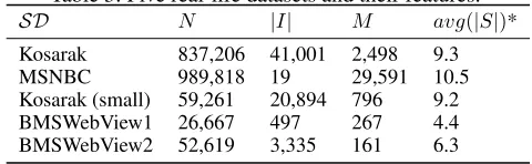
Table 3: Five real-life datasets and their features.
SD N |I| M avg(|S|)*
Kosarak 837,206 41,001 2,498 9.3
MSNBC 989,818 19 29,591 10.5
Kosarak (small) 59,261 20,894 796 9.2
BMSWebView1 26,667 497 267 4.4
BMSWebView2 52,619 3,335 161 6.3
*Average length of sequences
Numerical results
For our numerical tests, we use real-life click-stream bench-mark databases2, listed in Table 3. We note that two of these databases, Kosarak and MSNBC, are considerably larger than those typically reported in the CSPM literature, with about 900,000 sequences of length up to 29,500, and con-taining up to 40,000 items. None of these standard bench-mark datasets are annotated with attributes. To be able to evaluate our approach, we therefore generate three attributes of time, price, and quality, as follows. For the time attribute, we randomly generate a number between 0 and 600 seconds, to represent the time spent by users at each click. With a probability of 5%, we model the user leaving the session by setting the time between clicks to a value between 1 to 10 hours. For the price and quality attributes, we generate a number between 1 and 100 for each itemi∈S,∀S∈ SD.
All algorithms are coded in C++, with the exception of PPICt which is coded in Scala.3 All experiments are exe-cuted on the same PC with an Intel Xeon 2.33 GHz proces-sor, 24GB of memory, using Ubuntu 12.04.5 as operating system. We limit all tests to use one core of the CPU. The MPP code is available and open source.4
Comparison with prefix-projection and constraint
checks
Our first goal is to evaluate the impact of the MDD database and the associated constraint reasoning, especially in pres-ence of more complex constraints. However, no other CSPM system accommodates constraints such as average and me-dian and multiple item attributes. Because simple generate-and-test (via post-processing) does not scale due to the size of the databases, we developed a prefix-projection algo-rithm for the original database, that can handle multiple item attributes and effectively prune the search space for anti-monotone constraints such as gap and maximum span. We name this algorithm Prefix-Projection with Constraint Checks (PPCC). PPCC operates by prefix-projection and ex-tends a patternPif it satisfies all anti-monotone constraints, and prunes the extension otherwise. For non-monotone con-straints, PPCC extends infeasible patterns with the hope that a feasible super-pattern exists, and performs a constraint check at the end.
2
http://www.philippe-fournier-viger.com/spmf/index.php?link=datasets.php
3
We thank the developers of PPICt for sharing their code.
4
0.1 0.07 0.05 0.03 0.01 Min supp (%) 1
2 3
Time (sec)
Kosarak
103 PPCC3 MPP3 PPCC2 MPP2 PPCC1 MPP1
7 6 5 4 3
Min supp (%) 2
4 6
MSNBC
103
0.1 0.07 0.05 0.03 0.01 Min supp (%) 0
20 40
60 BMSWebView2
Figure 3: Mining with constraints 30 ≤ Cgap(time) ≤
900,900 ≤ Cspn(time) ≤ 3600,30 ≤ Cavg(price) ≤
70,40 ≤ Cmed(price) ≤ 60,40 ≤ Cavg(quality) ≤
60,30 ≤ Cmed(quality) ≤ 70. Attributes and their
corre-sponding constraints are added incrementally from 1 to 3.
In Figure 3 we compare the performance of MPP and PPCC in terms of total CPU time (MDD construction plus mining algorithm), given minimum support (Min supp) as a percentage of the total number of sequences. The experi-ment uses three scenarios with constraints on one, two, and three attributes, respectively:
time:30≤Cgap(time)≤900,900≤Cspn(time)≤3600, price:30≤Cavg(price)≤70,40≤Cmed(price)≤60,
quality:40≤Cavg(quality)≤60,30≤Cmed(quality)≤70.
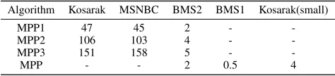
Scenario one (PPCC1 and MPP1) only considers the time constraints. Scenario two (PPCC2 and MPP2) considers the time and price constraints. Scenario three (PPCC3 and MPP3) considers all time, price, and quality constraints. The results in Figure 3 show that mining more constrained pat-terns takes more time for both methods. However, MPP is always more efficient than PPCC, and often considerably. For example, finding all frequent patterns with minimum support of 4% with all constraints (scenario three) in the MSNBC database takes PPCC about 4,000s while MPP only needs about 2,000s. Moreover, Table 4 shows that the time required to construct the MDD database and generate con-straint specific information is quite small. This indicates that our MDD database can be used to effectively and efficiently handle constraints such as average and median.
Comparison with PPICt
We next compare our approach to the state-of-the-art CSPM algorithm PPICt, which is implemented in the CP frame-work OscaR5(Aoga, Guns, and Schaus 2017). PPICt accom-modates a wide range of constraints, including gap and max-imum span constraints, but is restricted to a single attribute. We therefore evaluate MPP and PPICt for mining patterns with the following gap and maximum span constraints over the time attribute:
30≤Cgap(time)≤90, 900≤Cspn(time)≤3600.
Initial tests indicated that the PPICt code is unstable when executed on the full databases Kosarak and MSNBC. We therefore executed the codes on the smaller benchmark vari-ant of Kosarak (which is also used in (Aoga, Guns, and Schaus 2017)), BMSWebView1, and BMSWebView2. The results are presented in Figure 4, which follows the same format as Figure 3.
5
https://bitbucket.org/oscarlib/oscar/wiki/Home
0.1 0.07 0.05 0.03 0.01
Min supp (%)
0 200 400 600 800
Time (sec)
Kosarak (small)
PPICt PPCC MPP
0.1 0.07 0.05 0.03 0.01
Min supp (%)
0 20 40
60 BMSWebView1
0.1 0.07 0.05 0.03 0.01
Min supp (%)
0 20 40 60
80 BMSWebView2
Figure 4: Mining with one item attribute (time) and con-straints30≤Cgap(time)≤900, Cspn(time)≤3600.
Table 4: Time (in seconds) required for MDD construction and information generation.
Algorithm Kosarak MSNBC BMS2 BMS1 Kosarak(small)
MPP1 47 45 2 -
-MPP2 106 103 4 - -MPP3 151 158 5 -
-MPP - - 2 0.5 4
A first observation is that MPP and PPCC produce almost identical results, as they both benefit from the same prun-ing rules for anti-monotone constraints. The time required to build the MDD database, shown in Table 4, is made up by a faster prefix-projection algorithm due to implementing the gap constraints on the MDD itself. Both MPP and PPCC also outperform PPICt on Kosarak (small) and BMSWeb-view2, but all three methods perform similarly on BMSWe-bView1. However, PPICt uses significantly more memory, up to 14Gb, while MPP uses up to 1Gb, and PPCC con-sumes the lowest with at most 0.5Gb. We conclude that on this benchmark our approach is competitive with or more efficient than PPICt.
Conclusion
In this paper, we developed a novel MDD representation for CSPM. We prove how constraint satisfaction is achieved for a number of constraints, including sum, average, and me-dian, by storing constraint-specific information at the MDD nodes. Moreover, our approach is able to accommodate sev-eral item attributes with constraints, which occur frequently in real-world problems.
References
Agrawal, R.; Srikant, R.; et al. 1994. Fast algorithms for mining association rules. InProc. 20th int. conf. very large data bases, VLDB, volume 1215, 487–499.
Aoga, J. O. R.; Guns, T.; and Schaus, P. 2017. Min-ing time-constrained sequential patterns with constraint pro-gramming. Constraints1–23.
Bergman, D.; Cire, A. A.; van Hoeve, W.-J.; and Hooker, J. N. 2016.Decision Diagrams for Optimization. Springer. Bistarelli, S., and Bonchi, F. 2007. Soft constraint based pattern mining.Data & Knowledge Engineering62(1):118– 137.
Bonchi, F., and Lucchese, C. 2005. Pushing tougher con-straints in frequent pattern mining. InPAKDD, volume 5, 114–124. Springer.
Bonchi, F., and Lucchese, C. 2007. Extending the state-of-the-art of constraint-based pattern discovery.Data & Knowl-edge Engineering60(2):377–399.
Borah, A., and Nath, B. 2018. Fp-tree and its variants: To-wards solving the pattern mining challenges. InProceedings of First International Conference on Smart System, Innova-tions and Computing, 535–543. Springer.
Cambazard, H.; Hadzic, T.; and O’Sullivan, B. 2010. Knowledge compilation for itemset mining. InECAI, vol-ume 10, 1109–1110.
Chen, Y.-L., and Hu, Y.-H. 2006. Constraint-based sequen-tial pattern mining: The consideration of recency and com-pactness. Decision Support Systems42(2):1203–1215. Fournier-Viger, P.; Lin, J. C.-W.; Kiran, R. U.; Koh, Y. S.; and Thomas, R. 2017. A survey of sequential pattern min-ing.Data Science and Pattern Recognition1(1):54–77. Garofalakis, M. N.; Rastogi, R.; and Shim, K. 1999. Spirit: Sequential pattern mining with regular expression constraints. InVLDB, volume 99, 7–10.
Guns, T.; Dries, A.; Nijssen, S.; Tack, G.; and De Raedt, L. 2017. Miningzinc: A declarative framework for constraint-based mining.Artificial Intelligence244:6–29.
Han, J.; Pei, J.; Mortazavi-Asl, B.; Pinto, H.; Chen, Q.; Dayal, U.; and Hsu, M. 2001. Prefixspan: Mining sequen-tial patterns efficiently by prefix-projected pattern growth. Inproceedings of the 17th international conference on data engineering, 215–224.
Han, J.; Pei, J.; Yin, Y.; and Mao, R. 2004. Mining fre-quent patterns without candidate generation: A frefre-quent- frequent-pattern tree approach.Data mining and knowledge discovery 8(1):53–87.
Kemmar, A.; Loudni, S.; Lebbah, Y.; Boizumault, P.; and Charnois, T. 2016. A global constraint for mining sequential patterns with gap constraint. In International Conference on AI and OR Techniques in Constriant Programming for Combinatorial Optimization Problems, 198–215. Springer. Kemmar, A.; Lebbah, Y.; Loudni, S.; Boizumault, P.; and Charnois, T. 2017. Prefix-projection global constraint and top-k approach for sequential pattern mining. Constraints 22(2):265–306.
Le Bras, Y.; Lenca, P.; and Lallich, S. 2009. On optimal rule mining: A framework and a necessary and sufficient con-dition of antimonotonicity. In Pacific-Asia Conference on Knowledge Discovery and Data Mining, 705–712. Springer. Leung, C. K.-S.; Jiang, F.; Sun, L.; and Wang, Y. 2012. A constrained frequent pattern mining system for handling ag-gregate constraints. InProceedings of the 16th International Database Engineering & Applications Sysmposium, 14–23. ACM.
Lin, M.-Y., and Lee, S.-Y. 2005. Efficient mining of se-quential patterns with time constraints by delimited pattern growth.Knowledge and Information Systems7(4):499–514. Loekito, E., and Bailey, J. 2006. Fast mining of high dimen-sional expressive contrast patterns using zero-suppressed bi-nary decision diagrams. In Proceedings of the 12th ACM SIGKDD international conference on Knowledge discovery and data mining, 307–316. ACM.
Loekito, E., and Bailey, J. 2007. Are zero-suppressed bi-nary decision diagrams good for mining frequent patterns in high dimensional datasets? InProceedings of the sixth Aus-tralasian conference on Data mining and analytics-Volume 70, 139–150. Australian Computer Society, Inc.
Loekito, E.; Bailey, J.; and Pei, J. 2010. A binary decision diagram based approach for mining frequent subsequences. Knowledge and Information Systems24(2):235–268. Mallick, B.; Garg, D.; and Grover, P. S. 2014. Constraint-based sequential pattern mining: a pattern growth algorithm incorporating compactness, length and monetary. Int. Arab J. Inf. Technol.11(1):33–42.
Masseglia, F.; Poncelet, P.; and Teisseire, M. 2009. Ef-ficient mining of sequential patterns with time constraints: Reducing the combinations. Expert Systems with Applica-tions36(2):2677–2690.
Negrevergne, B., and Guns, T. 2015. Constraint-based se-quence mining using constraint programming. In Proceed-ings of CPAIOR, volume 9075 ofLNCS, 288–305. Springer. Nijssen, S., and Zimmermann, A. 2014. Constraint-based pattern mining. InFrequent pattern mining. Springer. 147– 163.
Pei, J.; Han, J.; and Wang, W. 2007. Constraint-based se-quential pattern mining: the pattern-growth methods. Jour-nal of Intelligent Information Systems28(2):133–160. Pyun, G.; Yun, U.; and Ryu, K. H. 2014. Efficient frequent pattern mining based on linear prefix tree.Knowledge-Based Systems55:125–139.
Soulet, A., and Cr´emilleux, B. 2005. Exploiting virtual patterns for automatically pruning the search space. In In-ternational Workshop on Knowledge Discovery in Inductive Databases, 202–221. Springer.