Numeric treatment of nonlinear second order multi-point boundary value problems using ANN, GAs and sequential quadratic programming technique Pages 431-442 Download PDF

(1)

* Corresponding author. Tel: +923009521379

doi: 10.5267/j.ijiec.2014.3.004

International Journal of Industrial Engineering Computations 5 (2014) 431–442

Contents lists available at GrowingScience

International Journal of Industrial Engineering Computations

homepage: www.GrowingScience.com/ijiec

Numeric treatment of nonlinear second order multi-point boundary value problems using ANN, GAs and sequential quadratic programming technique

Zulqurnain Sabira* and Muhammad Asif Zahoor Rajab

a

Department of Mathematics, Unique Science College (for girls) Dina, Pakistan

b

Department of Electrical Engineering, COMSATS Institute of Information Technology, Attock Campus, Attock Pakistan C H R O N I C L E A B S T R A C T

Article history:

Received December 2 2013 Received in Revised Format Mach 17 2014

Accepted March 24 2014 Available online March 29 2014

In this paper, computational intelligence technique are presented for solving multi-point nonlinear boundary value problems based on artificial neural networks, evolutionary computing approach, and active-set technique. The neural network is to provide convenient methods for obtaining useful model based on unsupervised error for the differential equations. The motivation for presenting this work comes actually from the aim of introducing a reliable framework that combines the powerful features of ANN optimized with soft computing frameworks to cope with such challenging system. The applicability and reliability of such methods have been monitored thoroughly for various boundary value problems arises in science, engineering and biotechnology as well. Comprehensive numerical experimentations have been performed to validate the accuracy, convergence, and robustness of the designed scheme. Comparative studies have also been made with available standard solution to analyze the correctness of the proposed scheme.

Artificial neural networks Genetic Algorithm Sequential Quadratic Programming Technique Hybrid computing techniques

1. Introduction

(2)

These multi-point BVPs are generally limited to second order equation. Agarwal and Kinguradze (Das et al., 2010) solved higher order linear ordinary differential equation with singularity at numerous points in 2004. Cheung and Ren (Das et al., 2010) discussed multi-point BVPs in 2005. Tatari and Dehghan (Das et al., 2010) used Adomian decomposition method (ADM) to find the solution of multi-point BVP in 2006. Gupta (1992, 1994, 1997) is believed to be the first who used functional analytical technique to demonstrate the existence of the solution monitored by Eloe and Henderson (1994), Ma (1999, 2001), Liu (2002), Webb (2001), etc. Deimling, (1985), Guo and Lakshmikantham (1988) and Krasnosel'skij (1964) used commonly fixed-point theorem on cones for positive solution. The source to apply this theorem can be initiated with semi linear elliptic equations on annuli (Erbe & Wang, 1994).

Stochastic numerical techniques have been used extensively by many researchers in different fields to solve linear and nonlinear differential equations (Raja & Samar, 2012; Khan, 2009). Interest in this area is significantly enhanced with effective numerical treatment for fractional differential equation (Khan et al., 2012). The analysis is carried out further by constructing different types of neural networks models with/without satisfying the boundary conditions, exactly. Furthermore, the effect of change on number on neurons on accuracy and convergence has also been analyzed.

In the present study, computational intelligent techniques are developed for solving a nonlinear multi-point BVPs representing to model the equation with the help of universal approximation capability of feed-forward artificial neural networks (ANN) trained in an unsupervised manner with genetic algorithms (GA) technique, as a tool for effective global search optimizer, hybrid with sequential quadratic programming technique (SQPT), an efficient local search approach. The proposed schemes are evaluated on four variants of the problems to validate the correctness of the approaches. The reliability and effectiveness of the proposed scheme is analyzed based on sufficient large set of data generated from independent execution of the optimizers, i.e., GA, SQPT and GA-SQPT.

The organization of the paper is as follows: in the second section, the system model of the problem is given in details. Design methodology consists of feed-forward artificial neural networks modeling and learning procedure based on GA, SQPT and GA-SQPT is narrated in section three. Numerical experimentation of number of variant of the problem is provided in section four. Concluding remarks and few future research directions are provided in the last section.

2. General form of Multi-point BVPs

Mathematically, this problem is a second-order ordinary differential equation (ODE). The generic form or general form of multi-point boundary value problems is written as follows,

2 2

1

( , ) ( ), 0 1,

(0) and (1) ( ) ,

m

i i

i d y

h y y q x x

dx

y A y y 







   

  

 _ _ _







(1)

where i(0,1),i0,1,2,...,m,and are constants

The Eq. (1) represents a standard form of multi-point BVP. The aim of studying the generalized form of the nonlinear multi-point BVP and its solutions is to develop a broader understanding of the general equations and to develop analytical tools to analyze these equations to cover more applications as they arise in the future.

3. Proposed Methodology

(3)

Z. Sabir and M. A. Zahoor Rajaa / International Journal of Industrial Engineering Computations 5 (2014)

3.1 Neural Network Mathematical Modeling

Mathematical model for the second order multi-point boundary value problems is constructed with the strength of feed-forward ANN, in the form of following continuous mapping for the solution y(x) , and its first dy/dx, second d2y/dx2 respectively, For the activation function log-sigmoid function

) 1 /( 1 )

(x e x

g    is used in the neural network modeling, given as:



 



2 ( ) 1 1 ( ) ( ) 1 1

2( ) ( )

2 2

2

2 2 ₍ ₎ 3 ₍ ₎ 2

1 1 ˆ ( ) ( ) , 1 ˆ ( ) , 1 ˆ 2 ( ) , 1 1 i i i i i i

i i i i i i i i

k n

i i i i w x

i i

w x

k n

i i i i i _{w x}

i i

w x w x

n

i i i i i

w x w x

i i

y x g w x

e

dy d e

g w x w

dx dx _e

d y d e e

g w x w

dx dx _e _e

                                                   _  _      



1 k             



(2)

where the vectors,wand are real-valued bounded unknown parameters, i.e., weights W = [,w,

], n is the number of neurons and g is the activation function generally taken as log-sigmoid function. The suitable combination of the networks given in the set (2) can be used to model the differential equation (1). An objective function or fitness function is developed in an unsupervised manner and it is defined by sum of two mean square error, e1 is error function associated with differential equation (1) and it is given as:

1 0 ), ( ), ( ˆ ˆ , 1 , ˆ ) ˆ , ˆ ( ˆ 1 1 2 2 2 1 2 1                           



 x mh x x q q x y y h N q dx y d y y h dx y d N e e e e m m m m m N m m m m m m (3)

Similarly, e2 is the error function associated with boundary conditions for Eq. (1) is given as:



2 2



0

2 (ˆ ) (ˆ )

2 1 B y A y

e    _N (4)

A second form of feed-forward artificial neural networks modeling is also constructed such that initial and boundary conditions are exactly satisfied in order to solve boundary value problems of the multi-point BVPs. The governing equations of alternative form of artificial neural networks model for the solution y(x), and its first dy/dx, second d2y/dx2 respectively, written as:

(4)

where ŷ(x), dŷ/dx, d2ŷ/dx2are the networks as shown in Eq. (6). The updated neural network can be developed for solving the general nonlinear multi-point boundary value problem (1) that satisfies boundary conditions exactly by taking the approximate values of P(x) and Q(x).

An objective function or fitness function is developed in an unsupervised manner for introducing error function base on the sum of mean square error as:

2 2

2 1 1

( , ) , (0,1)

1

, ( ), ( ),

N m

m m m

m

m m m m m

d y

h y y q x

N dx

N y y x q q x x mh

h





 _ _

       

 _ _

 

   

 



  

 

(6)

One can only deduce that with the availability of weights of neural networks such that the objective function given in Eq. (3) or Eq. (6) approaches zero, the proposed solution will approximate the exact solution of the problem closely.

3.2LearningMethodology

The procedure for training the designed parameters of the networks is accomplished with the help of genetic algorithms (GAs), sequential quadratic programming technique (SQPT) and hybrid computing approach GA-SQPT. The recent researches in genetic algorithms (GAs) has emphasized that the initial proposals were found incompetent of solving tough problems in a valuable and efficient way. For a large numbers of optimization problems, the time of execution of first-generation GAs increases significantly while solution quality decreases. Moreover the things such as selection schemes, encoding procedures, and self-adaptive and knowledge based operators play an important role in the optimization of well convex and stochastic nature problems. Since the beginning of the GAs, it has used for optimization of different fields of interest. In addition to the optimization problems, it is also used as an effective technique for achieving modeling, forecasting, control and simulation objectives. Traditional optimization approach start with a single candidate and search iteratively for the optimal result by using static heuristics. While, the GA techniques uses a population of candidate to seek a number of areas of a solution space, simultaneously and adaptively. The most famous methods that go beyond easy local search are GAs, simulated annealing (SA), and tabu search (TS) etc. Genetic algorithms work on a population of individuals. All individual is a potential solution to a given problem and is normally encoded as a fixed-length binary string, which is an analogy with an actual chromosome. After an initial population is randomly or heuristically generated, the algorithm evolves population through sequential and iterative application of selection, crossover, and mutation operators. A new generation is shaped after every each iteration. The strongest feature of the GA is that do not get stuck in local minimum.

Sequential quadratic programming techniques is basically a local search method which belongs to the class of efficient constrained optimization technique. The method is based on mathematical model for solving the Karush-Kuhn-Tucker (KKT) equations to get the desired Lagrange multipliers simply and consequently the global candidate solution. The SQP technique has been used in many practical important optimization problems since their origin. The interesting reader is referred to these literatures to known the history, importance, subject term, working and detail procedural step of the algorithm. The necessary procedure adopted for GA-SQPT is given in following steps:

Step 1: Initialization: Initial values of parameters are set in this step with random assignment and declarations. These setting are also tabulated in Table1 for important parameter of GAs.

Step 2: Fitness Evaluation: Calculate the fitness of each individual or chromosome of population using the Eq. (2) and Eq. (5), for first and second type of modeling, respectively.

Step 3: Termination Criteria: Terminate the algorithm when either of following criteria matches:

(5)

 Predefine number of generations are executed.

 Any of termination setting given in Table 1 for GA is fulfilled.

If termination criterion meets, then go to step 5

Step 4: Reproduction: Create next generation on the basis of Crossover: Call for scattered function, Mutation: Call for Adaptive Feasible function, Selection: Call for Stochastic Uniform function and Elitism account is set 4 etc.

Repeat the procedure from step 2 to step 4 with newly produced population

Step 5: Improvements: Sequential quadratic programming technique is used for further refinement of results by taking final adaptive weights of GAs as initial weights (start point) of SQPT algorithm. SQPT is applied as per setting of parameters given in Table 2. Store also the refined final weights of the algorithm.

Step 6: Neurons Analysis: Repeat step 1 to 5 for by taking size of initial weights, i.e. 15, 30 and 45 for k = 5, 10 and 15 neurons, respectively. These results are used for detail analysis of algorithm later.

The parameter setting used in this paper for GA algorithm in table 1 and SQPT algorithm are given in Table 2.

Table 1

Parameters Setting for GA in simulations

Parameters Setting Parameters Setting

Population Creation Linear feasible Bounds [-20, 20]

Initial Population range [-1, 1] Derivative Approximate by solver

Population 300 individuals TolFun 10-20

Generations 700 StallGenLimit 100

Scaling faction Rank Mutation Adaptive feasible

Selection function Stochastic Uniform Migration interval 20

Crossover fraction 0.80 Elite Count 02

Crossover function Heuristic TolCon 10-20

Migration fraction 0.2 Other Defaults

Table 2

Parameter Settings of “fmincon” function for SQPT in simulations

Parameters Settings/Values Parameters Settings/Values

Algorithm active-set Initial Weights best weights of GA

FinDiffType Central Initial Weight Vector length 30

TolX 10-20 Total Initial Weight Vectors 100

Iterations 700 Bounds ai, wi, bi ϵ (±20) ∀ i 1 to n

MaxFunEvals 200000 TolCon Zero

TolFun 10-20 Derivative Approximate by solver

TolCon 0 Other as defaults

3. Simulations and Results

(6)

Problem I: consider the following nonlinear multi-point boundary value problem (Das et al., 2010)

2 2 2 3 2 4 0 (1 )

( ) 2

2

1

(0) 0, y(1) 0.708667

1 5

i

d y x x dy

y x x

dx dx i y y i                _ _ _           



(7)

The exact solution of the problem is given as:

2

( )

y x x (8)

The proposed methodologies are applied to solve the problem by taking 10 neurons in the hidden layer of neural networks thus with a total 30 design parameter or weights, W( , , ) w .The fitness functions e and ε is formulated for this case for r ϵ (0, 1] with a step size h = 0.1 as:





2 2 2 1 0 2 3 2 1 2 4 2

0 1 0

0 2 2 2 1 0 2 3 2 1

ˆ (1 ) ˆ

1

ˆ 2

1 0 2

1 1

ˆ ˆ 0 .7 0 8 6 6 7

2 1 5

(1 )

1

2

1 0 2

m m m m

m m

m

i

m m m m

m m

m

d y x x d y

e y x

d x d x

i

y y y

i

d y x x d y

y x d x d x      _ _ _   _     _  _ _            _ _      _   _     _        _ _                 



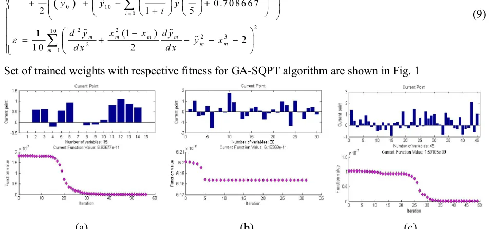
   (9)

Set of trained weights with respective fitness for GA-SQPT algorithm are shown in Fig. 1

(a) (b) (c)

Fig. 1. Set of optimal weights along with parameters for problem 1 by GA-SQPT using 5, 10 and 15 numbers of neurons

The proposed solution yˆ(x) and ~y(x) of the Eq. (7) is obtained using the optimal weights of algorithms in first equation of the set (2) and (5), respectively. The results due to GA-SQPT for the case k = 5 are given in simplify form as:

-(4.4035182757t-0.46497078475872) - 2.34877564743t 3.219305585838)

-(-0.4350829368t-2.29597874248666) -(0.5211

-3.67842896132752 1.14752400515832

ˆ _{( )}

( _{1 e}

1 e

2.39639235002620 2.35054880126743

1 e 1 e

GA SQPT

Y  x



 

 

 

  1789400447t-1.78365289124987) -(2.0465687282029t-4.25093661709093)

2.29409857048802 1 e

 

(10)

-(0 .5 91 393 77 19t-0 .6 17 416 04 556 1) -(0.53 95 227 15 24t-0 .9 35 460 476 65 )

-(-0.134 18 836 73 7t -0 .1 088 89 157 90 ) -(0

( ) ( 1)

-0 .0 0916 357 067 839 -0.20 873 044 9422 55

[

1 e 1 e

0.00 4556 410 854 91 0 .10 796 315 5614 23

1 e 1 e

G A SQ P

y  x x x x

           

.8 120 74 399 35 t 1.10 333 36 313 7) -(0.69 277 03 988 3t-0 .0 211 88 370 96 ) 0.865 239 3033 873

]

1 e

 



(7)

To find the solution of the problems, we have applied the GA, SQPT and hybrid approach GA-SQPT by invoking the Matlab built in functions using the parameters setting as given in Table 1 and Table 2.

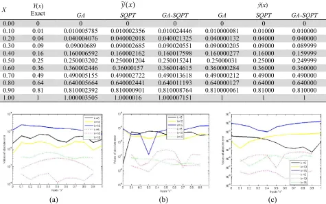
The results calculated for the both neural networks models optimized with GA-SQPT for different number of neurons, i.e., k = 5, 10 and 15, are given in the Table 3 for inputs t between 0 and 1 with a step size of 0.1. The results obtained with exact solution given in Eq. (8) are also given in the table for the same inputs. It is seen that the proposed solution match with exact solution to five to seven decimal space of the accuracy. The values of absolute error (AE) are determined for each algorithm, i.e., GA, SQPT and GA-SQPT, for both models and results are shown graphically in Fig 2

Table 3

Proposed results of the problem 1 using neural networks models with different neurons optimized with GA-SQPT

X Y(x)

Exact

) (

~_y _x _ŷ₍_x₎

GA SQPT GA-SQPT GA SQPT GA-SQPT

0.00 0 0 0 0 0 0 0

0.10 0.01 0.010005785 0.010002356 0.010024446 0.010000081 0.01000 0.010000

0.20 0.04 0.040004076 0.040002018 0.040021325 0.040000132 0.04000 0.040000

0.30 0.09 0.09000689 0.090002685 0.090020551 0.090000205 0.09000 0.089999

0.40 0.16 0.160006592 0.160002162 0.160017598 0.160000277 0.16000 0.159999

0.50 0.25 0.250003202 0.250001204 0.250015241 0.25000031 0.25000 0.249999

0.60 0.36 0.360002446 0.36000157 0.360014615 0.360000284 0.36000 0.360000

0.70 0.49 0.490005155 0.490002722 0.490013618 0.490000212 0.49000 0.490000

0.80 0.64 0.640005664 0.640002441 0.640011193 0.640000127 0.64000 0.640000

0.90 0.81 0.810002392 0.810000901 0.810008764 0.810000061 0.81000 0.810000

1.00 1 1.000003505 1.0000016 1.000007151 1 1 1

(a) (b) (c)

Fig. 2. Results based on AE for two models in case of problem I (solid and dotted lines for neural network with/without satisfying boundary condition exactly) (a) for GA (b) for SQP and (c) for GA-SQP

(8)

Problem II: Consider the following nonlinear multi-point boundary value problem (Das et al., 2010)

2

2 3 2

2

4

0

( ) 2 ( ) 2

1

(0) 0, y(1) 0.252

1 5

i

d y dy

xy x y x x x

dx dx

i

y y

i





    

  

   

 _ _ _

   

     





(12)

( ) ( 1)

y x x x (13)

The proposed methodologies are applied to solve the problem by taking 10 neurons in the hidden layer of neural networks thus with a total 30 design parameter or weights, W (,w, ). The fitness functions e and ε is formulated for this case for r ϵ (0, 1] with a step size h = 0.1 as:





2 2

1 0

2 3 2

2 1

2 4

2

0 1 0

0

2 2

1 0

2 3 2

2 1

ˆ ˆ

1

ˆ 2ˆ 2

1 0

1 1

ˆ ˆ 0 .2 5 2

2 1 5

1

2 2

1 0

m m

m m m m m

m

i

m m

m m m m m

m

d y d y

e x y y x x

d x d x

i

y y y

i

d y d y

x y y x x

d x d x





 _ _

  _      _

 _ _



 

      

 _ _

   

 _   _     _

   

 

 _ _



 



       



  





   

(14)

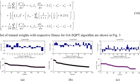
Set of trained weights with respective fitness for GA-SQPT algorithm are shown in Fig. 3

(a) (b) (c)

Fig. 3. Set of optimal weights along with parameters for problem 1 by GA-SQPT using 5, 10 and 15 numbers of neurons

The results due to GA-SQPT for the case k = 5 are given in simplify form as:

( 3 .3 4 6 4 8 7 2 4 8 t 2 .2 4 3 3 9 5 6 3 3 ) ( -0 .7 6 3 2 9 0 7 3 9 t -2 .4 6 8 2 0 9 5 2 ) ( -2 .4 8 3 1 5 4 9 3 6 t 2 .2 4 3 0 5 8 3 7 9 )

( 0 .6 3 6 5 6 6 5 8 7 t -1 .6 1 7 7 8 2 4 2 8 )

2 .2 0 8 8 3 6 5 5 5 0 .0 7 1 7 2 1 7 4 6 1 .8 1 0 7 3 4 9 0 8

ˆ _{( )}

1 e 1 e 1 e

2 .3 4 9 3 7 3 5 6 8 0 .2 0 9 6 8 0

1 e

G A S Q P

Y _ x  _   _

  

 

 (- 0 .7 7 5 2 1 7 6 4 1 t 0 .0 2 6 6 5 5 2 2 6 ) ( -0 .1 1 1 2 5 3 6 3 9 t 2 .6 9 7 6 9 5 2 1 4 )

( 2 .4 1 7 9 5 5 1 5 1 t -1 .8 3 6 7 7 2 0 2 2 ) (- 0 .0 0 5 2 2 7 5 0 3 t 3 .5 6 4 8 4 4 2 2 8 ) ( 2 .3 8 9 7 1 9 5 3 9 t -3 .9 0 5 7 3 1 6 6 4 )

3 8 7 1 .5 2 2 6 5 2 6 4 4

1 e 1 e

0 .7 8 9 9 5 5 0 8 2 0 .3 9 4 0 0 7 7 5 2 1 .1 2 8 6 7 6 5 3 4

1 e 1 e 1 e

 





 

  

  

(1 .6 9 4 9 8 2 9 4 t -5 .1 2 1 4 1 1 8 0 5 )

2 .3 4 3 5 5 7 9 8

1 e

 

(9)

2

(0.472487834t-0.246514322) (0.095063987t-0.487915835)

(-0.305821484t 0.2 63233801) (0.944712492t 0.484968391)

( ) ( 1)

-0.216506509 0.109795413

[

1 e 1 e

0.482970033 0.018294812

1 e 1 e

0.23071701 GA SQP

y  x x x x x

 

   



 

 

 

 

(0.3 16310172t-0.346091359) (-0.201150105t 0.031234018)

(-0.69348194t 0.274893474) (0.842677833t 0.550224316)

(-0.576745358t -0.000596585)

1 0.426353657

1 e 1 e

0.427353059 0.28357977

1 e 1 e

0.230940307 0.

1 e



 





 

 

 

 

 (0.529882133t-0.372938855)

250772371 ] 1e

(16)

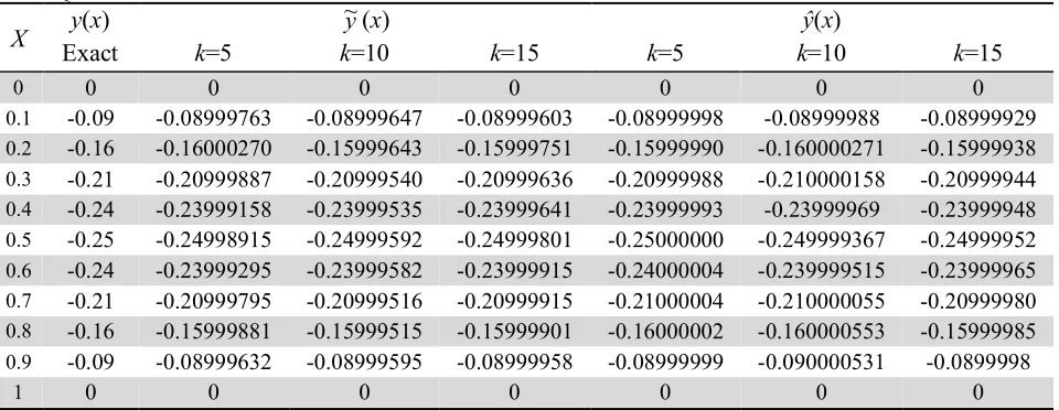
The results obtained for the both neural networks models of GA-SQPT for k = 5, 10 and 15, are also presented in the Table 4 along with exact solution using Eq. (13).

Table 4

Proposed results of the problem using neural networks models with different neurons optimized with GA-SQPT

X y(x) ~ (y x) ŷ(x)

Exact k=5 k=10 k=15 k=5 k=10 k=15

0 0 0 0 0 0 0 0

0.1 -0.09 -0.08999763 -0.08999647 -0.08999603 -0.08999998 -0.08999988 -0.08999929

0.2 -0.16 -0.16000270 -0.15999643 -0.15999751 -0.15999990 -0.160000271 -0.15999938

0.3 -0.21 -0.20999887 -0.20999540 -0.20999636 -0.20999988 -0.210000158 -0.20999944

0.4 -0.24 -0.23999158 -0.23999535 -0.23999641 -0.23999993 -0.23999969 -0.23999948

0.5 -0.25 -0.24998915 -0.24999592 -0.24999801 -0.25000000 -0.249999367 -0.24999952

0.6 -0.24 -0.23999295 -0.23999582 -0.23999915 -0.24000004 -0.239999515 -0.23999965

0.7 -0.21 -0.20999795 -0.20999516 -0.20999915 -0.21000004 -0.210000055 -0.20999980

0.8 -0.16 -0.15999881 -0.15999515 -0.15999901 -0.16000002 -0.160000553 -0.15999985

0.9 -0.09 -0.08999632 -0.08999595 -0.08999958 -0.08999999 -0.090000531 -0.0899998

1 0 0 0 0 0 0 0

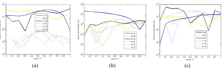
The values of absolute error AE are determined for each algorithm, i.e., GA, SQPT and GA-SQPT for both models and results are shown graphically in Fig 4.

(a) (b) (c)

(10)

Problem III: Consider the following nonlinear multi-point boundary value problem (Das et al., 2010)





2 2

4

0

( ) cos 1 sin

1

(0) 0, y(1) 0.3277

1 5

i

d y dy

y x x x

dx dx i y y i              _ _ _           



(17)

( ) sin

y x  x (18)

The proposed methodologies are applied to solve the problem by taking 10 neurons in the hidden layer of neural networks thus with a total 30 design parameter or weights, W (,w,). The fitness functions e and ε is formulated for this case for r ϵ (0, 1] with a step size h = 0.1 as:





2 2 1 0 2 1 2 4 2 0 10 0 2 2 10 2 1 ˆ ˆ 1

ˆ (cos 1) sin

1 0

1 1

ˆ ˆ 0.32 77

2 1 5

1

(cos 1) s in

10

m m

m m m

m

i

m m

m m m

m

d y dy

e y x x

d x dx

i

y y y

i

d y d y

y x x

dx d x      _ _         _ _            _ _      _   _     _        _ _               



   (19)

The proposed solution yˆ(x) and ~y(x) of the Eq. (17) is obtained using the optimal weights of algorithms in first equation of the set (2) and (5), respectively. The results due to GA-SQP for the case

k = 15 are given in simplify form as:

(-2.768026281t-0.07889657) (1.577421678t 0.764886671) (-2.261775246t 1.861122461) (-0.069874053t-1.296706406)

-0.081445879 1.033908368 1.99603985 1.159325859 ˆ _{( )}

1 e 1 e 1 e 1 e

0.298371

GA AST

Y _ x   _  _ 

   

 _{(-0.764074296t-0.48929052)} _{(1.329328249t-1.775691856)} _{(-0.452390437t-0.437945435)} _{(-0.69183918t-0.116530885)}

(-0.337217405t-076 2.389750629 0.408425054 1.081451478

1 e 1 e 1 e 1 e

1.118420805 1 e        

 1.205051142) (0.335142006t 0.432716274) (-3.539588497t-0.950303091) (0.200102379t-0.184532206)

(0.608412449t 0.339126605)

0.4761533 0.899806552 0.418222187

1 e 1 e 1 e

0.262434241 0.337546906

1 e 1



  

  

 

  (-2.253966554t-0.045011958) (0.432918626t 0.136772046)

0.18163671

e 1 e_ 

(20)

2

(0.7 58 597 56 4t-0.910 34 693 ) (-0.3 241 78 31 1t-0.3 61 743 89 4)

(-0.2 57 77 147 2t-0.794 77 99 84) (0 .01 17 30 42

0 .5 6 40 10 4 55 0 .5 3 49 50 7 38 ( ) 0.1 58 5 27 38 4 ( 1) [

1 e 1 e

0 .33 23 2 07 15 0 .3 92 07 9 39 2

1 e 1 e

G A S Q P

y _ x  x  xx x  

 

 

 



4 t-0.3 108 11 71 7) (0.021 41 86 74t-0 .92 711 76 35 ) (-0.219 92 67 12t0 .69 57 73 998 )

(-0.321 41 89 36t 0 .27 368 47 92 ) (-0.2 78 016 42 6t-0.1 66 833 51 2)

0 .12 6 89 37 9 5 0 .66 6 05 93 0 2

1 e 1 e

0.4 38 33 2 40 4 0.3 37 7 76 68 9 0.2 46

1 e  1 e

 

 

  

  (-0.0 753 88 87 3t-0.2 50 126 43 8) -(1 .17 14 317 08 t-0 .50 71 70 459 )

(-0 .40 61 609 24 t-0 .19 53 00 395 ) (0 .47 739 27 6t 0.196 94 245 5) (0 .22 61 94 5

6 01 32 4 0 .35 0 45 34 0 9

1 e 1 e

0 .12 8 86 21 8 4 0.2 65 02 7 02 9 0 .59 6 50 27 9 2

1 e 1 e  1 e



 

  

   73 t-0.3 539 44 16 7) (0.527 98 11 59t 0 .85 634 49 39 )

(1 .62 35 271 8t 0.59 062 77 88)

0.4 53 4 71 33 8 1 e

0 .7 7 35 46 9 68

] 1 e       (21)

(11)

Table 4

Proposed results of the problem using neural networks models with different neurons optimized with GA-SQPT

X

y(x) ~y(x) ŷ(x)

Exact k =5 k=10 k=15 k=5 k=10 k=15

0 0 0 0 0 0 0 0

0.1 0.099833 0.099827 0.099832 0.099834 0.099832 0.099834 0.099835

0.2 0.198669 0.198665 0.198668 0.19867 0.198669 0.198669 0.198671

0.3 0.29552 0.295515 0.295519 0.295521 0.29552 0.295521 0.295522

0.4 0.389418 0.389416 0.389417 0.389419 0.389418 0.38942 0.389421

0.5 0.479426 0.479425 0.479425 0.479426 0.479426 0.479428 0.479429

0.6 0.564642 0.564642 0.564642 0.564644 0.564644 0.564645 0.564646

0.7 0.644218 0.644216 0.644217 0.644219 0.644219 0.64422 0.64422

0.8 0.717356 0.717356 0.717356 0.717358 0.717357 0.717357 0.717358

0.9 0.783327 0.78333 0.783327 0.783329 0.783328 0.783328 0.783328

1 0.841471 0.841473 0.841472 0.841473 0.841473 0.841473 0.841473

The values of absolute error AE are determined for each algorithm, i.e., GA, SQP and GA-SQP for both models and results are shown graphically in Fig 5 as follows,

(a) (b) (c)

Fig. 5. Results based on AE for two models in case of problem III (solid and dotted lines for neural network with/without satisfying boundary condition exactly) (a) for GA (b) for SQPT and (c) for GA-SQPT

4. Conclusions

Following conclusions are drawn for our research studies:

 A new soft computing approach has been developed effectively for solving multi-point boundary value problems, in-particularly multi-point BVPs and its variants using neural networks optimized with genetic algorithm, sequential quadratic programming technique and their hybrid combination.

 The sufficient low value of absolute error has established the correctness of the designed scheme.

 By taking fewer number of neurons, the performance of method were efficient for finding the solution, however, it increased the number of neurons, one can get slightly more accurate solution with immense reliability but at the cost of more computations.

Future research directions

Following are few suggested research directions for interested readers:

 One can look for more accurate neural networks modeling by using alternate activation functions like radial basis, Mexican Hat, wavelets hat, etc.

(12)

 Better hardware platform like parallel, grid and cloud computing, can help in decreasing computational time of the algorithm, considerably. Consequently, we may look for other complicated nonlinear problems to solve by our design scheme.

Acknowledgement

Authors like to thank the anonymous referees for constructive comments on this paper.

References

Cannon, J. R. (1984). The one-dimensional heat equation, volume 23 of Encyclopedia of Mathematics and its Applications.

Cannon, J. R., Esteva, S. P., & Van Der Hoek, J. (1987). A Galerkin procedure for the diffusion equation subject to the specification of mass. SIAM Journal on Numerical Analysis, 24(3), 499-515. Deimling, K. (1985). Nonlinear Functional Analysis. Springler-Verlag, Berlin.

Das, S., Kumar, S., & Singh, O. P. (2010). Solutions of Nonlinear Second Order Multi-point Boundary Value Problems by Homotopy Perturbation Method. Applied Mathematics: An International

Journal, 5(10), 1592-1600.

Erbe, L. H., & Wang, H. (1994). On the existence of positive solutions of ordinary differential equations. Proceedings of the American Mathematical Society, 120(3), 743-748.

Gupta, C. P. (1992). Solvability of a three-point nonlinear boundary value problem for a second order ordinary differential equation. Journal of Mathematical Analysis and Applications, 168(2), 540-551. Gupta, C. P. (1994). A note on a second order three-point boundary value problem. Journal of

Mathematical Analysis and Applications, 186(1), 277-281.

Gupta, C. P., & Trofimchuk, S. I. (1997). A sharper condition for the solvability of a three-point second order boundary value problem. Journal of Mathematical Analysis and Applications, 205(2), 586-597.

Guo, D., & Lakshmikantham, V. (1988). Nonlinear Problems in Abstract Cones (Vol. 5). San Diego: Academic press.

Eloe, P. W., & Henderson, J. (1994). Multipoint boundary value problems for ordinary differential systems. Journal of Differential Equations, 114(1), 232-242.

Ilin, V. A., & Moiseev, E. I. (1987). Nonlocal boundary-value problem of the first kind for a Sturm-Liouville operator in its differential and finite difference aspects. Differential Equations, 23(7), 803-810. Khan, J. A., Zahoor, R. M. A., & Qureshi, I. M. (2009, December). Swarm intelligence for the solution

of problems in differential equations. In Environmental and Computer Science, 2009. ICECS'09.

Second International Conference on (pp. 141-147). IEEE.

Khan, A., Raja, M. A. Z., & Ijaz Mansoor Qureshi, J. (2012). An application of evolutionary computational technique to non-linear singular system arising in polytrophic and isothermal sphere. Global Journal of Researches In Engineering, 12(1-I).

Krasnosel'skij, M. A. (1964). Positive solutions of operator equations (p. 381). L. F. Boron (Ed.). Groningen: P. Noordhoff.

Liu, B. (2002). Positive solutions of a nonlinear three-point boundary value problem. Computers &

Mathematics with Applications, 44(1), 201-211.

Ma, R. (1999). Positive solutions of a nonlinear three-point boundary-value problem. Electronic

Journal of Differential Equations, 1999(34), 1-8.

Ma, R. (2001). Positive solutions for second-order three-point boundary value problems. Applied

Mathematics Letters, 14(1), 1-5.

Raja, M. A. Z., & Samar, R. (2012). Neural network optimized with evolutionary computing technique for solving the 2-dimensional Bratu problem. Neural Computing and Applications, 1-12.

Timoshenko, S. P., & Gere, J. M. (1961). Theory of elastic stability. 1961.