Volume 35 - Article 18 | Pages 505–534

(1)

DEMOGRAPHIC RESEARCH

VOLUME 35, ARTICLE 18, PAGES 505

−

534 PUBLISHED 26 AUGUST 2016

http://www.demographic-research.org/Volumes/Vol35/18/ DOI: 10.4054/DemRes.2016.35.18

Research Article

Fertility progression in Germany:

An analysis using flexible nonparametric cure

survival models

Vincent Bremhorst

Michaela Kreyenfeld

Philippe Lambert

This open-access work is published under the terms of the Creative Commons Attribution NonCommercial License 2.0 Germany, which permits use, reproduction & distribution in any medium for non-commercial purposes, provided the original author(s) and source are given credit.

(2)

1 Introduction 506

2 Context and previous research 508

3 Methods and data 510

3.1 Methods and research strategy 510

3.1.1 Cure survival models 510

3.1.2 Bayesian inference 512

3.2 Data 513

3.2.1 Sample 513

3.2.2 Dependent variable: transition to a second and a third child 514

3.2.3 Independent variables 515

4 Results 517

4.1 Second births 517

4.2 Third births 523

4.3 Comparison with a Cox model 526

5 Discussion 527

6 Acknowledgements 529

(3)

Fertility progression in Germany:

An analysis using flexible nonparametric cure survival models

Vincent Bremhorst1

Michaela Kreyenfeld2,3 Philippe Lambert1,4

Abstract

OBJECTIVE

This paper uses data from the German Socio-Economic Panel (GSOEP) to study the transition to second and third births. In particular, we seek to distinguish the factors that determine the timing of fertility from the factors that influence ultimate parity progression.

METHODS

We employ cure survival models, a technique commonly used in epidemiological studies and in the statistical literature but only rarely applied to fertility research.

RESULTS

We find that education has a different impact on the timing and the ultimate probability of having a second and a third birth. Furthermore, we show that the shape of the fertility schedule for the total population differs from that of ‘susceptible women’ (i.e., those who have a second or a third child).

CONCLUSION

Standard event history models conflate timing and quantum effects. Our approach overcomes this shortcoming. It estimates separate parameters for the hazard rate of having a next child for the ‘susceptible population’ and the ultimate probability of having another child for the entire population at risk.

1_{Université catholique de Louvain, Institut de Statistique, Biostatistique et Sciences Actuarielles, Voie du} Roman Pays 20, B-1348 Louvain-la-Neuve, Belgium. E-Mail: [email protected].

2_{Hertie School of Governance GmbH Friedrichstraße 180, 10117 Berlin, Germany.}

(4)

CONTRIBUTION

We go beyond standard cure survival models, also known as split population models, used in fertility research by specifying a flexible non-parametric model using Bayesian P-splines for the latent distribution (related to the timing of an extra birth) instead of a parametric model. Our approach is, so far, limited to time-constant covariates, but can be extended to include time-varying covariates as well.

1. Introduction

Event history models have a long tradition in demographic research. They represent a bridge between the classical life table methods and modern regression techniques (Hoem 1993). Unlike OLS regression, they are able to account for censoring and allow for a flexible specification of the baseline intensity and the integration of time-varying covariates into the analysis (Rizopoulos 2012). In fertility research, the most commonly used models are proportional hazard specifications, such as the piecewise exponential or the Cox model. Although they are widely used, these models have a serious shortcoming: They are unable to separate the impact of the covariates on the timing of births from the factors that influence the ultimate parity progression. As they cannot differentiate between timing and quantum, they often produce misleading results.

(5)

educated women are more likely to progress to higher order births, or whether they simply space their births closer together than other women. Our paper addresses the call for more “real-world justifications” (Ní Bhrolcháin 2011: 850) that show that it is worthwhile to separate the level and timing of fertility.

(6)

In all of the abovementioned studies, a parametric distribution was specified to model the time to an extra birth. In this paper, we model the transition to the next child using a flexible non-parametric model, based on Bayesian P-splines (Bremhorst and Lambert 2016). Flexible nonparametric modeling was used by demographers before: For example, Gayawan and Adebayo (2013) used Bayesian P-splines to model the baseline and the non-linear effects in an extended Cox model when studying the age at first birth in Nigeria, while calibrated splines were specified by Schmertmann (2012) to obtain a flexible estimation of the fertility schedule from abridged data. In this work, we employ post-estimation procedures to visualize the baseline intensities for the total population and the ‘susceptible’ women (those who had another child). Most importantly, our estimates show that the fertility schedules of the two populations differ considerably. This finding has major implications for standard event history modeling. It suggests that the shape of the baseline intensity in standard event history models is very sensitive to the size of the ‘immune’ population.

The paper is structured as follows: In Section 2 we provide background information on birth dynamics in Germany and summarize previous research that examined the link between education and fertility. In Section 3 we describe the methodology and the data. We use data from the German Socio-Economic Panel to investigate the transition to second and third births. As our method is unable (so far) to handle time-varying covariates, we do not study the progression to first birth. Many important covariates (such as education) may be treated as time-constant covariates in second and third birth models (they can be fixed at the start of the process), while this is not reasonable for the analysis of first births. In Section 4 we first discuss the results from the promotion time model and provide graphical representations that highlight the importance of distinguishing timing from quantum in the analysis of birth dynamics. Then a comparison with the results given by a classical Cox model is presented. In Section 5 we conclude by discussing the strengths and the limitations of the promotion time model. The main advantage of this model is that it is able to separate timing from quantum effects, while a significant limitation of the model is that its methodology is designed for time-constant covariates only. Finally, we discuss how the model could be extended to enable the inclusion of time-varying covariates.

2. Context and previous research

(7)

in 1930 had a fertility rate of 2.1, and thus a rate that was around replacement level. For the cohorts born around 1965, this value declined to 1.5 (Pötzsch 2010; Human Fertility Database 2015). An important component of the low fertility levels in (western) Germany is the rather high share of women who remain childless. About 22 percent of (western) German women who are now approaching the end of their reproductive period will remain childless (Kreyenfeld and Konietzka 2016). It is well known that in eastern Germany the total fertility rate fell sharply after German reunification, to below one. Recently, the period birth rates in eastern and in western Germany have again reached parity (Goldstein and Kreyenfeld 2011). In addition to gathering data on total fertility, the Federal Statistical Office of Germany now also collects information on biological birth order and spacing. According to these vital statistics data, in 2010 the mean length of time between the first and the second birth was around four years in western Germany and five years in eastern Germany, while the average length of time between the second and the third birth was 4.8 years in western Germany and 5.4 years in eastern Germany (Pötzsch 2012). The vital statistics do not, however, provide information on exposure rates or on birth behavior by socioeconomic subgroup, such as by educational attainment.

(8)

parity progression. Thus, event history researchers have argued about the correct interpretation of their findings.

3. Methods and data

3.1 Methods and research strategy

3.1.1 Cure survival models

Cure survival models extend classical time-to-event models when an unknown fraction of the population under study never experience the event of interest; they enable the simultaneous estimation of the quantum and of the timing of the monitored event. Two main families of models can be distinguished: the mixture and the non-mixture (also referred to as the promotion time model) cure models. The mixture cure model, first introduced by Berkson and Gage (1952) and extensively studied in the statistical literature afterward (see Peng and Dear 2000; Peng 2003; Lu 2010 among others), defines the population survival function as a mixture of contributions due to the susceptible and the non-susceptible sub-populations:

𝑆𝑝(𝑡) = (1− 𝜋) +𝜋𝑆𝑠(𝑡), (1)

where π denotes the probability of being susceptible and 𝑆𝑠(𝑡) is the survival function

of the susceptible subjects. In this work we focus on the second family. The promotion time model was first motivated by the biological mechanism in the development of cancer (Yakovlev and Tsodikov 1996; Tsodikov 1998; Chen, Ibrahim, and Sinha 1999): The model assumes that each subject is exposed to N ~ P(𝜃) (Poisson distributed) independent latent factors (corresponding to carcinogenic cells in cancer studies) with a time to detection (of a tumor generated from a given cell) having a common proper distribution function F(t). The time-to-event is defined as the minimum of the N latent event times. However, its motivation can easily be translated in the realm of fertility studies. Indeed, when studying the transition to second or third birth, a latent factor could be seen as a potential decisive argument to decide to have an additional child and the ‘time for its detection’ as the time required for it to be convincing. It is assumed that the latent factors (or potential decisive arguments) are all defined at the onset of the process (i.e., directly after the birth of the previous child) without possibility of an evolution of their number during the follow-up of the subject. Then, the population survival function of the promotion time model can be shown to be

(9)

𝑆𝑝(𝑡) = exp[−𝜃𝐹(𝑡)]. (2)

The probability of never having a second (third) child is given by:

P[N = 0] = exp (−θ). (3)

The independent variables, measured at the beginning of the follow-up and denoted by x and z, enter the model through a log-link on parameter 𝜃 (which increases with the probability of having a second or third child) and a Cox model for the latent distribution F(t) (related to the timing of an extra birth):

𝜃(𝒙) = exp (𝛽0+ 𝛽1𝑥1+⋯+𝛽𝑝𝑥𝑝); (4)

𝐹(𝑡|𝒛) = 1− 𝑆0(𝑡)exp (𝜆1𝑧1+⋯+𝜆𝑞𝑧𝑞). (5)

As pointed out by Bremhorst and Lambert (2016), covariate vectors x and z can share some components and remain identifiable provided that the follow-up of the study is sufficiently long. In practice, if the Kaplan-Meier estimate of the survival function shows a plateau in the right tail of the distribution, then the sufficiently long follow-up assumption is respected.

In this work, the logarithm of the baseline hazard function ℎ0(𝑡), which yields the

baseline survival function 𝑆0(𝑡) in the Cox model, is specified using a linear

combination of a large number of cubic B-splines combined with a roughness penalty on finite differences of adjacent B-spline coefficients to force smoothness (Eilers and Marx, 1996, 2010):

log�ℎ0(𝑡)�= ∑𝑘=1𝐾 𝜑𝑘𝑏𝑘(𝑡) and 𝜏 ∑𝑘(𝛥𝑟𝜑𝑘)2 , (6)

where {𝑏𝑘(. ),𝑘= 1, … ,𝐾} denotes the cubic B-splines basis associated with a

predefined number of equidistant knots on the follow-up interval and 𝜏 is the penalty parameter. For identification purposes, the last spline coefficient is set to an arbitrarily large enough value (say, 10) to force 𝑆�0(.) to be virtually 0 at the end of the follow-up

(Bremhorst and Lambert, 2016).

The model specification provides a flexible and smooth estimation of the population hazard function ℎ𝑝(𝑡) and of the hazard function ℎ𝑠(𝑡) of the susceptible

(10)

ℎ𝑝(𝑡) = 𝜃𝑓(𝑡) and ℎ𝑠(𝑡) =_𝑆_𝑝₍_𝑡₎𝑆_−exp𝑝(𝑡)₍_−𝜃₎ℎ𝑝(𝑡), (7)

where 𝑓(𝑡) is the latent density function.

3.1.2 Bayesian inference

Instead of working with a penalized likelihood, in the Bayesian framework the roughness penalty enters through the multivariate normal prior distribution of the spline coefficients (Lang and Brezger 2004):

𝝋 ~ 𝑵𝑲(𝟎,𝜏𝝋′𝑷𝝋), (8)

where 𝐏=𝐃’𝐃 + ε𝑰𝒌 is a full rank matrix for some small quantity εand D is the rth

order difference matrix. For the penalty parameter 𝜏, the robust prior distribution suggested by Jullion and Lambert (2007) is specified :

𝜏 | 𝛿 ~ 𝐺(𝜈₂,𝜈𝛿₂) and 𝛿 ~𝐺(𝑎𝛿,𝑏𝛿), (9)

where 𝐺(𝑎,𝑏) defines a Gamma distribution with mean 𝑎_𝑏. Because it can be shown that 𝜈 has a posterior distribution close to the uniform when 𝑎𝛿 =𝑏𝛿 are small enough

(0.0001, say), fixing 𝜈 (equal to 2, for example) has no impact on the shape of the survival curve. Independent normal distributions with a large variance are used as priors for each regression coefficient.

The results presented in Tables 3 and 5 were obtained using MCMC with chains of length 150,000, including a burn-in of 50,000, with parameter estimates given by the median of their posterior sample. The chains were generated using adaptive multivariate Metropolis steps for the spline and the regression coefficients (Haario, Saksman and Tamminen 2001; Atchadé and Rosenthal 2005). Gibbs steps are used to sample from the posterior of the penalty parameters 𝜏 and 𝛿 because their conditional posterior distributions belong to the Gamma family:

𝜏 | 𝝋,𝛿,𝑫 ~ 𝐺(𝜈+𝐾₂ ,𝜈𝛿+𝝋₂′𝑷𝝋) and 𝛿 | 𝜏,𝑫 ~𝐺 �𝑎𝛿+𝜈₂ ,𝑏𝛿+𝜈𝜏₂�. (10)

(11)

1992; Brooks and Gelman, 1998). More information on Bayesian analysis can be found e.g., in Gelman et al. (2013).

3.2 Data

3.2.1 Sample

The data for the following analyses are from the German Socio-Economic Panel (v31.0) (Wagner, Frick, and Schupp, 2007).5_{The German Socio-Economic Panel (GSOEP) is a}

representative panel study for Germany. The first wave of this survey was launched in 1984, and the respondents have been interviewed on an annual basis since then. Over time, the GSOEP has been extended through the addition of various subsamples. Most importantly, an oversample of the eastern German population was added to the survey in 1990. Migrants and foreigners are also overrepresented. As analyzing the fertility of migrants and of eastern Germans would have required us to conduct a separate investigation, we limited our investigation to German nationals who were born in and are currently living in western Germany.6_{It should be noted that individual respondents}

may have entered or left our study population if their location or citizenship changed. We have also restricted our sample to female respondents, as in the GSOEP the fertility histories of women are more reliable than those of men. However, the characteristics of each woman’s co-residential partner, and particularly his (or, if the woman is in a same-sex union, her) educational attainment, are accounted for in our analysis. The sample is further restricted to women who were still of childbearing age (17–49) when they entered the panel. Respondents were censored after the maximum duration of 180 months (15 years) after they had their first and their second child, or when they dropped out of the survey. Respondents who dropped out of the panel after participating in the survey for just one year were eliminated as well, as they could not contribute any exposure time to our study. Twins births were not considered in the analysis for the same reason. Cases with invalid birth histories or missing information on educational attainment were also omitted from the sample. As our focus in this study is on second and third births, we further restricted our investigation to respondents who were at risk of having a second or a third child. Left-truncated cases were also

5_{The data that we used for this analysis is available in the SOEP-archive for reanalysis of published findings:}

https://www.diw.de/en/diw_01.c.340860.en/soep_reanalyses.html. R programs for replicating this paper’s results are available upon request from the authors.

6_{The SOEP includes an additional high income subsample that was drawn in 2002. We also removed this}

(12)

eliminated. Thus, only respondents who had a first or a second child after they entered the panel study are used in our analysis. We also eliminated the few cases with missing information on the month of childbirth. The final sample comprises 1406 female respondents at risk of a second birth, of whom 674 reported having had a second child (before censoring). There were 1186 women at risk of having a third child, of whom 219 gave birth to a third child (before censoring).

3.2.2 Dependent variable: transition to a second and a third child

We have monthly information on second and third births. The process time for the second birth is the elapsed time since the birth of the first child (measured in months). The process time for the third birth is the elapsed time since the second birth. For the censored cases, the process time is the duration since the last birth until censoring.

(13)

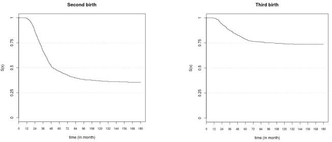
Figure 1: Transition probabilities to second and third births (Kaplan‒Meier survival estimates)

Source: SOEP 1984–2013, (v31.0), only Germans living in western Germany, high income sample was excluded.

3.2.3 Independent variables

Our data span the period 1984–2013. We have organized the data into person-month formats. The analyses include time-constant covariates only, which are ‘frozen’ at the time of the onset of the process. For example, for the analysis of the second birth, we employ information on the educational level and the partnership status at the first birth. For the third birth models, all of the covariates take the value at the birth of the second child. As we mentioned in Section 3.1, the probability of (never) having an additional child is modeled through the mean number of latent factors (cf. eq. 3). Since the promotion time model assumes that the latent factors occur only at the beginning of the study, it would not be reasonable to let the time dependent covariates influence this probability.

(14)

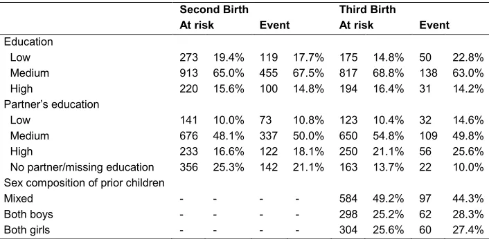
The control variables are age at the first birth and calendar period. Both are employed as a continuous covariate. For the third birth, we also controlled for the spacing of the first two births using a continuous variable that depicts the length of time between the previous two births. Tables 1 and 2 display by parity the descriptive statistics of the categorical and continuous independent variables, respectively. It should be noted that only a small fraction of women were partnered with a man who had a low level of education. This pattern may be the result of less educated men having lower chances than better educated men of entering a co-residential union (Bastin 2016).

Table 1: Descriptive statistics of the independent categorical variables for all mothers at risk of an extra birth (column ‘At risk’) or restricted to women who were reported to have an additional child (column ‘Event’)

Second Birth Third Birth

At risk Event At risk Event

Education

Low 273 19.4% 119 17.7% 175 14.8% 50 22.8%

Medium 913 65.0% 455 67.5% 817 68.8% 138 63.0%

High 220 15.6% 100 14.8% 194 16.4% 31 14.2%

Partner’s education

Low 141 10.0% 73 10.8% 123 10.4% 32 14.6%

Medium 676 48.1% 337 50.0% 650 54.8% 109 49.8%

High 233 16.6% 122 18.1% 250 21.1% 56 25.6%

No partner/missing education 356 25.3% 142 21.1% 163 13.7% 22 10.0%

Sex composition of prior children

Mixed - - - - 584 49.2% 97 44.3%

Both boys - - - - 298 25.2% 62 28.3%

Both girls - - - - 304 25.6% 60 27.4%

(15)

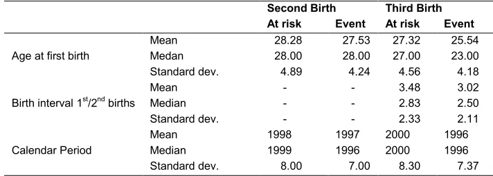
Table 2: Descriptive statistics of the independent continuous variables (in year) for all mothers at risk of an extra birth (column ‘At risk’) or restricted to women who were reported to have an additional child (column ‘Event’)

Second Birth Third Birth

At risk Event At risk Event

Age at first birth

Mean 28.28 27.53 27.32 25.54

Medan 28.00 28.00 27.00 23.00

Standard dev. 4.89 4.24 4.56 4.18

Birth interval 1st_/2nd_births Mean _Median - _- - _- 3.48 _2.83 3.02 _2.50

Standard dev. - - 2.33 2.11

Calendar Period

Mean 1998 1997 2000 1996

Median 1999 1996 2000 1996

Standard dev. 8.00 7.00 8.30 7.37

4. Results

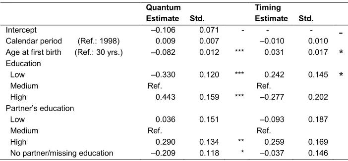
4.1 Second births

Table 3 shows the regression parameters for the transition to a second birth. A positive value for the estimate in the quantum column (cf. β in eq. 4) means that the probability of having an additional child increases when the corresponding covariate takes a positive value and the other covariates are fixed. A positive value for the estimate in the timing column (cf. 𝝀 in eq. 5) means that the transition to a second birth tends to happen sooner for a susceptible woman (again, for a positive value of the covariate and fixed values of the others).

(16)

However, relative to having a medium educated partner, having a highly educated partner was associated with a significantly greater probability of having a second child. The high birth rates of the university graduates could indicate that a high income of both men and women is a prerequisite for having a second child. However, in a male breadwinner regime such as Germany, it comes as a surprise that women’s labor market potential supports fertility transitions. An alternative explanation is a “selection argument” (Kreyenfeld 2002; Bartus et al. 2013). In a context where work and family life is incompatible, university educated women will remain childless to a greater extent than less educated women. Those who decide for a first child may be more family-prone than other women, an aspect that will accelerate their progression to a second child. Another explanation could be that we are unable to fully eliminate the strong effect of the partner’s high education on fertility, because of the substantial educational homogamy that exists in western Germany.

Table 3: Transition to a second birth – Results from cure survival models

Quantum Timing

Estimate Std. Estimate Std.

Intercept –0.106 0.071 - - -

_-

Calendar period (Ref.: 1998) 0.009 0.007 –0.010 0.010

Age at first birth (Ref.: 30 yrs.) –0.082 0.012 *** 0.031 0.017

_*

Education

Low –0.330 0.120 *** 0.242 0.145

_*

Medium Ref. Ref.

High 0.443 0.159 *** –0.277 0.202

Low 0.036 0.151 –0.093 0.187

Medium Ref. Ref.

High 0.290 0.134 ** 0.259 0.169

No partner/missing education –0.209 0.118 * –0.037 0.146

Source: SOEP 1984–2013, (v31.0), only Germans living in western Germany, high income sample was excluded. Signif. codes: * = 0.1 ; ** = 0.05 ; *** = 0.01

(17)

level have any significant influence on fertility timing.In previous research, it has been stipulated that highly educated women (and potentially also men) need to squeeze their births into a shorter period of time, because they start their childbearing career later than less educated individuals (Kreyenfeld 2002; Bartus et al. 2013). Also the argument by Ní Bhrolcháin (1986) of a “work-accelerated childbearing” would suggest that timing effects are very important for highly educated women. However, our results do not support this hypothesis.

The left-hand graph of Figure 2 shows the population hazard function (when all covariates were set at their reference values) with its 95 percent pointwise credible interval. For the whole population (women who were or were not susceptible), this function quantifies the evolution over time of the instantaneous risk of having a second child immediately after the considered time (for the women still at risk of second pregnancy). The right-hand graph of Figure 2 shows the hazard function of susceptible women (i.e., the women who will have a second child), and suggests a peak at about 3.5 years after the birth of the first child. It should be noted that as more than 90 percent of the second births occurred within 5.5 years of the first birth, the hazard functions are plotted only on this time interval (as we might otherwise be tempted to over-interpret the shape of the estimated hazard functions later on, despite the large underlying uncertainties). As expected, we find that the instantaneous risk of having a second child was higher for susceptible mothers than for the whole population. We can also see that the shapes of the two graphs differ. While the population hazard suggests that second birth intensities increased at around two to three years after the first birth, the hazard for the susceptible women peaked later.

(18)

Figure 2: Transition to a second birth. The fitted population hazard function (left) and the fitted hazard function of the susceptible mothers (right) with 95% pointwise credible intervals when all covariates are set at their reference values

What is the substantive meaning of the difference? Did second birth rates peak two to three years after the first birth, or did they peak later? To answer that question, let us assume for a moment that the ‘immune population’ are people who, for biological reasons, could not have a second child. If we accept that interpretation, the immune population should have been excluded from the representation because they were not at risk of childbearing. Thus, the figure on the right would represent the ‘true’ second birth profile. In reality, the people who never had a second child are a heterogeneous population, consisting, for example, of people who were unable to have another child for biological reasons, as well as of people who simply never fulfilled (for one reason or another) their desire to have another child. If we accept that interpretation, the latter group should not be removed from the risk population. It would therefore follow that the figure on the left represents the true fertility schedule. Whatever the correct assessment of the nature of the immune population, it is important to acknowledge that the fertility schedule can be strongly influenced by the inclusion or exclusion of the immune population.

(19)

higher educational level was associated with an increased conditional probability of having a second child (upper panel, left). Among the women who had a second child, those with the lowest educational level tended to have their second child more quickly than other women (right-hand graph). It should be noted that the suggested differences only became relevant two years after the birth of the first child. The lower row of Figure 3 illustrates the effect of the partner’s educational level (for the fixed reference value of the other covariates). The left-hand graph confirms that a woman whose partner had a university degree had a greater conditional probability of having a second child (more than one year after the first birth). However, the differences suggested by the lower right-hand graph turned out to be not significant (at the 10 percent credibility level).

(20)

Figure 3: Transition to a second birth. The fitted population hazard function (left), the fitted hazard function for the susceptible mothers (right). All covariates are set at their reference values, except the educational level of the mother (row 1) and of her partner (row 2)

(21)

Table 4: Probabilities of a second birth (in %). The estimates correspond to the posterior medians

Women’s education Partner’s education Estimate 95% C.I.

Low Low 48.9 [ 37.9 ; 60.9 ]

Medium Low 60.6 [ 50.1 ; 71.1 ]

High Low 76.6 [ 62.5 ; 88.5 ]

Low Medium 47.7 [ 39.2 ; 56.6 ]

Medium Medium 59.3 [ 54.2 ; 64.5 ]

High Medium 75.3 [ 64.6 ; 85.7 ]

Low High 57.9 [ 46.7 ; 69.2 ]

Medium High 69.9 [ 61.1 ; 78.1 ]

High High 84.6 [ 74.9 ; 92.5 ]

4.2 Third births

(22)

groups on the labor market or the ‘high earning potentials’ advance to births of higher order (Kreyenfeld 2002; Kreyenfeld and Andersson 2014). To buttress that claim it would be useful to include labor market earnings into the analysis. Furthermore, there are many other confounding factors that mitigate the relationship, among them values and attitudes that strongly correlate with educational attainment. Neither can we rule out that selectivity explains some of the findings. Lower educated men are more likely to remain childless. If they father a child, they often do not move in with a partner (Bastin 2016). Because we only observe the male partner’s characteristics if he lives with the respondent, we may catch a selective group of committed low educated men.

Table 5: Transition to a third birth – Results from cure survival models

Quantum Timing

Est Std Est Std

Intercept –1.968 0.156 - - - -

Calendar period (Ref : 1998) –0.004 0.011 –0.022 0.013 *

Age at first birth (Ref : 30 yrs) –0.126 0.021 *** 0.016 0.028

Birth interval 1st_/2nd_{births (Ref : 3 yrs)} _–0.203 _0.040 _*** _{0.081 0.043 *}

Mix Ref. Ref.

Both boys 0.176 0.173 –0.034 0.204

Both girls 0.192 0.174 –0.228 0.211

Education

Low 0.214 0.190 –0.092 0.242

Medium Ref. Ref.

High 0.112 0.239 0.070 0.287

Low 0.521 0.224 ** –0.309 0.302

Medium Ref. Ref.

High 0.717 0.192 *** 0.349 0.244

No partner/missing education 0.091 0.253 0.427 0.312

(23)

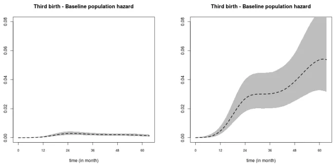
Figure 4 displays the hazard functions for the population (on the left) and for the susceptible mothers, i.e., women who will have a third child, (on the right) when all covariates are set at their reference values. Because only 18.5% of the sample had a third birth, the population at instantaneous risk of having a third child was, not surprisingly, rather small. If we look at the susceptible mothers only, we can see that the instantaneous risk of having a third child increased steeply during the first two years and grew more slowly thereafter. The shape of the estimated hazard function becomes more difficult to interpret over 4.5 years due to the growing uncertainty. Nevertheless, the shape of the graph shows that up to five years after the second birth, the birth hazard increased gradually. The population hazard (graph on the left) shows a rather flat pattern between ages two and five. Unfortunately, the sample sizes for third births were too small to allow us to present the graphs by level of education.

Figure 4: Transition to a third birth. The fitted population hazard function (left) and the fitted hazard function of the susceptible mothers (right) with 95% pointwise credible intervals when all covariates are set at their reference values

(24)

couples in which the man has the highest earning potential (measured by his high level of education) and the woman has the lowest opportunity costs of childrearing (measured by her low level of education) have the greatest chances of having a large family. This interpretation is, however, at odds with the finding that highly educated couples were also very likely to have three children. If both partners had earned a university degree, their probability of having three children was 27.4%. Less educated couples had a slightly lower probability, 25.3%, of having three children. Meanwhile, the medium educated couples were at a relative disadvantage: Their chances of having a third child were only around 13%. Thus, they were less than half as likely to have a third child as the highly and the less educated couples.

Table 6: Probabilities of a third birth (in %). The estimates correspond to the posterior medians

Women’s education Partner’s education Estimate 95% C.I.

Low Low 25.3 [ 15.2 ; 39.4 ]

Medium Low 21.0 [ 13.3 ; 31.9 ]

High Low 23.2 [ 13.1 ; 38.3 ]

Low Medium 15.9 [ 10.0 ; 23.8 ]

Medium Medium 13.0 [ 09.7 ; 17.1 ]

High Medium 14.4 [ 08.8 ; 22.4 ]

Low High 29.7 [ 19.0 ; 44.3 ]

Medium High 24.8 [ 17.6 ; 34.2 ]

High High 27.4 [ 18.5 ; 38.2 ]

4.3 Comparison with a Cox model

One of the main assumptions of the Cox model is that all women under study will sooner or later give birth to an additional child. Looking at the Kaplan‒Meier estimate of the survival function given in Figure 1, it is clear that this assumption is not supported when studying the transition to second and third births in West Germany. Nevertheless, Table 7 shows the results of a classical Cox model fitted using the coxph

(25)

for the effect of age at first birth on second parity progression as well as for the effect of the time elapsed between the first two children on the transition to third birth. The Cox model results also point out that women with a low or high educated partner have a larger third birth rate compared to women with a medium educated partner. However, one cannot distinguish whether this significant effect is due to the timing or to the probability of the event while this issue is immediately highlighted by the promotion time model. This conclusion holds for high educated one child mothers compared to medium educated ones. As expected, if a factor has no significant influence on the probability and on the timing of an extra birth, the effect of this factor remains non-significant under the Cox model (for example, see the effect of the women’s educational attainment on third parity progression).

Table 7: Transition to second and third births. Results from the Cox model

Second Births Third Births

LHR Std. LHR Std.

Calendar period (Ref : 1998) 0.005 0.006 –0.011 0.010

Age at first birth (Ref : 30 yrs) –0.073 0.010 *** –0.119 0.019 ***

Birth interval 1st/₂nd_{child (Ref : 3 yrs)} _- _- _{- –0.183} _{0.039 ***}

Mix - - - Ref.

Both boys - - - 0.153 0.164

Both girls - - - 0.139 0.166

Education

Low –0.240 0.112 ** 0.171 0.182

Medium Ref. Ref.

High 0.336 0.123 *** 0.133 0.228

Low 0.001 0.131 0.423 0.212 **

Medium Ref. Ref.

High 0.399 0.116 *** 0.872 0.188 ***

No partner/missing education –0.244 0.105 ** 0.216 0.238

Source: SOEP 1984–2013, (v31.0), only Germans living in western Germany, high income sample was excluded. Signif. codes : * = 0.1 ; ** = 0.05 ; *** = 0.01

5. Discussion

(26)

of models enabled us to distinguish the factors that influence the probability of having an additional child from those that influence the timing of an additional birth. We went beyond standard cure survival models by specifying a flexible non-parametric model (using Bayesian P-splines) for the specification of the baseline intensity. Our main factor of interest was the influence of female and male education on parity progression. The results of our investigation show that the ultimate probability of having a second child increased with the level of education of the mother, but also that less educated women had their second child sooner than their better educated counterparts. When we looked at third births, we found that a woman with a highly educated partner was more likely to have had an additional child. Neither female nor male educations levels were, however, shown to have a significant influence on the spacing of the third birth.

We have also demonstrated that the shape of the fertility schedule differs depending on whether we examine the entire population or only the ‘susceptible women’ (those who eventually experience the event). For second births, for example, the ‘full population hazard’ suggests that birth intensities peak around three years after the first birth. If we focus on the susceptible women, the peak shifts by one year. While this change in the fertility schedule may be obvious for bio-statisticians, for applied researchers it has major implications for the correct interpretation of the baseline intensities of an event history model. The age (or duration) when birth intensities peak is commonly interpreted as being the point in time when it is most likely that a woman will have a child. The validity of this interpretation is arguable when the population considered at risk includes women who will never experience the event of interest. Indeed, as the share of this immune population grows over time, the peak of the fertility schedule shifts, even if the population who experience the event of interest does not change its behavior.

It is widely known in the research community that standard event history models conflate timing and quantum effects. Hence, it is surprising to observe that alternative model specifications that try to separate out the two have still not seeped into applied fertility research. An illustration of possible misleading conclusions from the classical time-to-event model was presented in Section 4.3 by comparing the results obtained from the Cox and from the promotion time models.

(27)

6. Acknowledgments

(28)

References

Alter, G., Oris, M., and Tyurin, L. (2007). The shape of a fertility transition and analysis of birth intervals in Eastern Belgium. Paper presented to the Population Association of America meeting in New York.

Atchadé, Y.F. and Rosenthal, J.S. (2005). On adaptive Markov chain Monte Carlo algorithms. Bernoulli 11(5): 815–828. doi:10.3150/bj/1130077595.

Bastin, S. (2016). Partnerschaftsverläufe alleinerziehender Mütter: Eine quantitative Untersuchung auf Basis des Beziehungs- und Familienpanels. Wiesbaden: Springer VS. doi:10.1007/978-3-658-10685-0.

Bartus, T., Murinkó, L., Szalma, I., and Szél, B. (2013). The effect of education on second births in Hungary: A test of the time-squeeze, self-selection, and partner-effect hypotheses. Demographic Research 28(1): 1–32. doi:10.4054/DemRes.2013.28.1.

Bauer, G. and Jacob, M. (2010). Fertilitätsentscheidungen im Partnerschaftskontext: Eine Analyse der Bedeutung der Bildungskonstellation von Paaren für die Familiengründung anhand des Mikrozensus 1996–2004 [Fertility decisons in the partnership context: An analysis of the educational constellations of couples for family formation based on the microcensus 1996–2004]. Kölner Zeitschrift für Soziologie und Sozialpsychologie 62: 31–60. doi:10.1007/s11577-010-0089-y. Beaujouan E. and Solaz A. (2013). Racing against the biological clock? Childbearing

and sterility among men and women in second unions in France. European Journal of Population 29(1): 39–67. doi:10.1007/s10680-012-9271-4.

Begall, K. and Mills, M.C. (2012). The influence of educational field, occupation, and occupational sex segregation on fertility in the Netherlands. European Sociological Review 28(4): 1–23. doi:10.1093/esr/jcs051.

Berinde, D. (1999). Pathways to a third child in Sweden. European Journal of Population 15: 349–378. doi:10.1023/A:1006287630064.

Berkson, J. and Gage, R. (1952). Survival curve for cancer patients following treatment.

Journal of the Americal Statistical Association 47: 501–515. doi:10.1080/016 21459.1952.10501187.

(29)

Bremhorst, V. and Lambert, P. (2016). Flexible estimation in cure survival models using Bayesian P-splines. Computational Statistics and Data Analysis 93: 270– 284. doi:10.1016/j.csda.2014.05.009.

Brooks, S. and Gelman, A. (1998). General methods for monitoring convergence of iterative simulations. Journal of Computational and Graphical Statistics 7: 434– 455.

Chen, M.-H., Ibrahim, J.G., and Sinha, D. (1999). A new bayesian model for survival data with a surviving fraction. Journal of the American Statistical Association

94: 909–919. doi:10.1080/01621459.1999.10474196.

Chi, Y. and Ibrahim, J. G. (2006). Joint models for multivariate longitudinal and multivariate survival data. Biometrics 62(2): 432–445. doi:10.1111/j.1541-0420.2005.00448.x.

Eilers, P. and Marx, B. (1996). Flexible smoothing with B-splines and penalties (with discussion). Statistical Modeling 11(2): 89–121.

Eilers, P. and Marx, B. (2010). Splines, knots, and penalties. Wiley Interdisciplinary Reviews: Computational Statistics 2(6): 637–653. doi:10.1002/wics.125.

Gayawan, E. and Samson B.A. (2013). A Bayesian semiparametric multilevel survival modelling of age at first birth in Nigeria. Demographic Research 28(45): 1339– 1372. doi:10.4054/DemRes.2013.28.45.

Gelman, A. and Rubin, D. (1992). Inference from iterative simulation using multiple sequences. Statistical Science 7(4): 457–511. doi:10.1214/ss/1177011136. Gelman, A., Carlin, J.B., Stern, H.S., Dunson, D.B., Vehtari, A., and Rubin, D. (2013).

Bayesian data analysis.3rd_{ed. Boca Raton: Chapman and Hall/CRC.}

Gerster, M., Keiding, N., Knudsen, L.B., and Strandberg-Larsen, K. (2007). Education and second birth rates in Denmark 1981–1994. Demographic Research 17(8): 181–210. doi:10.4054/DemRes.2007.17.8.

Geweke, J. (1992). Evaluating the accuracy of sampling-based approaches to calculating posterior moments. In: Bernardo, J., Berger, J., David, A., and Smith, A. (eds.). Bayesian statistics 4. Oxford: Clarendon: 169–193.

(30)

Gottard, A., Mattei, A., and Vignoli, D. (2015). The relationship between education and fertility in the presence of a time varying frailty component. Journal of the Royal Statistical Society, Series A 178(4): 863–881. doi:10.1111/rssa.12097.

Gray, E., Evans, A., Anderson, J., and Kippen, R. (2010). Using split-population models to examine predictors of the probability and timing of parity progression.

European Journal of Population 26(3): 275–295. doi:10.1007/s10680-009-9201-2.

Haario, H., Saksman, E. and Tamminen, J. (2001). An adaptive Metropolis algorithm.

Bernoulli 7(2): 223–242. doi:10.2307/3318737.

Hoem, J.M. (1993). Classical demographic methods of analysis and modern event-history techniques. Stockholm Research Reports in Demography75. Stockholm: Stockholm University.

Huinink, J. (1989). Das zweite Kind: Sind wir auf dem Weg zur Ein-Kind-Familie? [The second child: Are we on the path towards the one-child-family?].

Zeitschrift für Soziologie 18(3): 192–207.

Human Fertility Database. (2015). Cohort fertility: West Germany. Max Planck Institute for Demographic Research (Germany) and Vienna Institute of Demography (Austria). Available at www.humanfertility.org (data downloaded on July, 16 2015).

Jullion, A. and Lambert, P. (2007). Robust specification of the roughness penalty prior distribution in spacially adaptive Bayesian P-splines models. Computational Statistics and Data Analysis 51(5): 2542–2558. doi:10.1016/j.csda.2006.09.027. Kravdal, Ø. (2001). The high fertility of college educated women in Norway: An

artefact of the separate modelling of each parity transition. Demographic Research 5(6): 187–215. doi:10.4054/DemRes.2001.5.6.

Kreyenfeld, M. (2002). Time squeeze, partner effect or self-selection? An investigation into the positive effect of women’s education on second birth risks in West Germany. Demographic Research 7(2): 15–48. doi:10.4054/DemRes.2002.7.2. Kreyenfeld, M. and Andersson, G. (2014). Socio-economic differences in the

unemployment and fertility nexus in cross-national comparison. Advances in Life Course Research 21: 59–73. doi:10.1016/j.alcr.2014.01.007.

(31)

Kreyenfeld, M. and Konietzka, D. (2016). Childlessness in Germany. In: Kreyenfeld, M. and Konietzka, D. (eds.). Childlessness in Europe: Context, causes and consequences. Wiesbaden: Springer.

Lang, S. and Brezger, A. (2004). Bayesian P-splines. Journal of Computational and Graphical Statistics 13(1): 183–212. doi:10.1198/1061860043010.

Li, L. and Chloe, M. (1997). A mixture model for duration data: Analysis of second births in China. Demography 34(2): 189–197. doi:10.2307/2061698.

Lu, W. (2010). Efficient estimation for an accelerate failure time model with a cure fraction. Statistica Sinica 20: 661–674.

McDonald, J.W. and Rosina, A. (2001). Mixture modelling of recurrent event times with long-term survivors: Analysis of Hutterite birth intervals. Statistical Methods and Applilcations 10(1): 257–272.

Milewski, N. (2010). Fertility of immigrants: A two-generational approach in Germany. Berlin: Springer. doi:10.1007/978-3-642-03705-4.

Ní Bhrolcháin, M. (1986). Women’s paid work and the timing of births: Longitudinal evidence. European Journal of Population 2(1): 43–70. doi:10.1007/BF0 1796880.

Ní Bhrolcháin, M. (2011). Tempo and the TFR. Demography 48(3): 841–861. doi:10.1007/s13524-011-0033-4.

Nitsche, N., Matysiak, A., Van Bavel, J., and Vignoli, D. (2015). Partners’ educational pairings and fertility across Europe. Families and Societies working paper 2015/38. Stockholm: Families and Societies/University of Stockholm.

Oláh, L.S. (2003). Gendering fertility: Second births in Sweden and Hungary.

Population Research and Policy Review 22(2): 171–200. doi:10.1023/A:1025 089031871.

Oppermann, A. (2014). Exploring the relationship between educational field and transition to parenthood: An analysis of women and men in Western Germany.

European Sociological Review 30(6): 728–749. doi:10.1093/esr/jcu070.

Peng, Y. (2003). Estimating baseline distribution in proportional hazards cure models.

Computional Statistics and Data Analysis 42(1–2): 187–201. doi:10.1016/S0 167-9473(02)00158-5.

Peng, Y. and Dear, K. (2000). A nonparametric mixture model for cure rate estimation.

(32)

Pötzsch, O. (2010). Cohort fertility: A comparison of the results of the official birth statistics and of the microcensus survey 2008. Comparative Population Studies

35(1): 185–204.

Pötzsch, O. (2012). Geburtenfolge und Geburtenabstand: Neue Daten und Befunde [Birth order and birth spacing: New data and new evidence]. Wirtschaft und Statistik 2: 89–101.

Prskawetz, A. and Zagaglia, B. (2005). Second births in Austria. Vienna Yearbook of Population Research 3: 143–170.

Rizopoulos, D. (2012). Joint models for longitudinal and time-to-event data with applications in R. Boca Raton: Chapman and Hall/CRC. doi:10.1201/b12208. Schmertmann, C.P. (2012). Calibrated spline estimation of detailed fertility schedules

from abridged data. MPIDR Working Paper 2012–022. Rostock: Max Planck Institute for Demographic Research.

Tesching, K. (2012). Education and fertility: Dynamic interrelations between women’s educational level, educational field and fertility in Sweden. [PhD thesis]. Stockholm: Stockholm University. http://www.demogr.mpg.de/publications/ files/4565_1334049671_1_Full%20Text.pdf.

Tsodikov, A.D. (1998). A proportional hazard model taking account of long-term survivors. Biometrics 54(4): 1508–1516. doi:10.2307/2533675.

Upchurch, D.M., Lillard, L.A., and Panis, C.W.A. (2002). Nonmarital childbearing: Influences of education, marriage, and fertility. Demography 39(2): 311–329. doi:10.1353/dem.2002.0020.

Wagner, G.G., Frick, J.R., and Schupp, J. (2007). The German Socio-Economic Panel Study (SOEP): Scope, evolution and enhancements. Schmollers Jahrbuch 127: 139–169. doi:10.2139/ssrn.1028709.

Yamaguchi, K. and Ferguson, L. (1995). The stopping and spacing of childbirths and their birth-history predictors: Rational choice theory and event history analysis.

American Sociological Review 60(2): 272–298. doi:10.2307/2096387.