ON MODELING TRACES IN A COMPUTING ENVIRONMENT FOR HUMAN LEARNING BASED INDICATORS

WIND SPEED FORECASTING USING REPTREE AND

BAGGING METHODS IN KIRKLARELI-TURKEY

1_{METIN ZONTUL,} 2_{FATIH AYDIN,} 3_{GOKHAN DOGAN,} 4_{SELCUK SENER,} 5_{OGUZ KAYNAR} 1_{Department of Software Engineering, Istanbul Aydin University, Turkey}

2

Department of Software Engineering, Kirklareli University, Turkey

3_{Vocational School of Technology and Science, Kirklareli University, Turkey} 4_{Vocational School of Anadolu Bil, Istanbul Aydin University, Turkey}

5_{Department of Management Information Systems, Cumhuriyet University, Sivas, Turkey}

E-mail: [email protected], [email protected], [email protected] 4_{[email protected],} 5_{[email protected]}

ABSTRACT

In this study, an analysis was performed by examining the wind power potential of Kırklareli province which is in the west of Turkey. Statistical data between 2001 and 2007 was used in this study. The data was obtained from Kırklareli branch of State Meteorological Service. In Kırklareli region, wind speed forecasts regarding the year 2013 were made for windpower plants that are supposed to be built. WEKA tool was used for the performed analyzes. Algorithm which was used for forecasting is REPTree which is decision tree algorithm. There are two basic reasons to use REPTree algorithm. First, it produces better results compared to other machine learning methods, and secondly, the model produced with REPTree has a clear content. For this reason, new information can be gathered by using the tree model. This advantage of REPTree algorithm is combined with Bagging method and average model is generated by using the models produced by new training sets that are derived from the original training set. In this way, the model that will provide the highest accuracy rate is produced. The correlation coefficient value between the real and estimated values is obtained as 0,8154 by applying cross-validation method on the training set. This shows that REPTree can be used along with Bagging method for the wind speed forecasting of the year 2013.

Keywords:Wind Speed Forecast, Machine Learning, Bagging, REPTree, Time Series Analysis

1. INTRODUCTION

In today’s world, energy is amongst most important values. Traditional energy production methods, which are unable to meet the needs of population with developing economy, have begun to enter into a bottleneck in terms of sustainability. Green energy concept has quickly become a sort of resource that replaces fossil fuels dating from early 2000s. Wind power, as one of the green energy sources, has an increased share all over the world recently. By the year 2004, the amount of wind energy production over the world is 47.693 MW [1]. By the end of the first half of the year 2012, this has increased to 254.000 MW [2]. One of the main problems for developed countries as from the beginning of 2000s is to produce natural, low-cost, efficient and clean energy [3]. As for our country, this figure does not have any discrepancies as well and the need is gradually getting bigger. With its industrial economy and rapidly growing population, Turkey has an increasing need for energy, too. By the year 2050, the population of Turkey is expected

to be 94.585.000 [4]. Therefore, for the planning of energy production; efficient use of energy, research and development of alternative energy sources right along with available energy sources have a great importance. Turkey’s renewable energy sources, country in general and for various region’s resource assessments have recently been the subject of national and international literature. These studies are about; the environment, energy policy and the social aspects of sustainability of renewable energy [5], the current state of available fossil fuel resources [4], recommendations on using these sources more effective (cogeneration systems), present state of the situation [5] and statistical approaches and [6,7] reports. In addition, wind power potential of many regions in Turkey was examined in these studies. Ranking of geographical regions in Turkey upon wind power potential is made as following; Marmara, North-West Black Sea and Aegean Coasts [8].

Systems) System. In addition, in the study of Gokcek and others [10], annual average power density of the region was calculated using Weibull and Rayleigh probability density functions.

Various forecasting models are used for wind speed forecasting. Artificial neural networks are among the most commonly used models. The artificial neural network model which is developed by Erdil et al. [11] for meteorological forecasts performs well regarding the forecast results. Apart from artificial neural network models, ANFIS is one of the most commonly used systems. Models formed by ANFIS are hybrid models. These models perform well when solving very complex problems [12]. Aside from these models, quite new models are also used and one of these techniques is Evolutionary Product Unit Neural Networks (EPUNN). Just like ANFIS system, EPUNN method also forms hybrid models. In addition, methods formed by EPUNN are quite good in comparison with standard artificial neural network models. Moreover, an interpretation is also possible about non-linear relation that is predicted by the model which is formed by EPUNN [13]. In this study, methods with different approaches were used for wind speed forecasting, as well. These methods are machine learning algorithms that produce different models by creating different approaches about the data. Among these algorithms, Bagging classifier produces a meta-model using a machine learning classifier, k nearest neighbour classifier produces a stagnant model, Radial Basis Function Network classifier produces an artificial neural network model, REPTree produces a model based decision tree and ZeroR classifier produces a majority-based approach model.

As specified in Turkey Ministry of Energy and Natural Resources Wind Power Plants Specifications, at least 6 months before setting up a wind power plant and 12 months of feasibility analysis should be made. Yet, according to these specifications, the data should be measured within maximum 1 hour of intervals, and should include strength and direction information of wind. In this study, average speed and direction information which is obtained with one hour intervals of 10 meter high metering stations through seven years (2001, 2002, 2003, 2004, 2005, 2006, and 2007) by General Directorate of State Meteorology Affairs in Kırklareli province.

In the study, wind power potential of Kırklareli province is analyzed using statistical data regarding

the dates between 2001 and 2007, and wind speed predictions for 2013 are performed. Predictions, which are made using training data, are performed by WEKA tool which contains several machine learning algorithms.

Machine learning (ML) is a field of study that aims to give computers the ability to learn without programming [14]. ML is widely used for the implementation of inferential algorithm which is one of the steps of knowledge discovery [15]. Inductive ML algorithms can learn patterns within labeled data, namely the data which has a given output [16].

2. CLASSIFICATION ALGORITHMS USED IN THE EXPERIMENTS

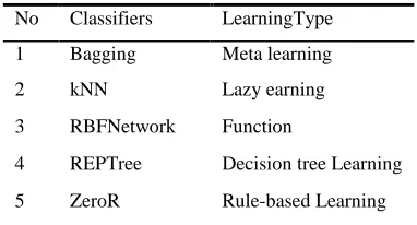
ML algorithms within WEKA (Waikato Environment for Knowledge Analysis) constitute a model for training data by applying several different strategies. In the study, it is determined to use five different learning algorithms by the software called WEKA workbench. These algorithms are shown in Table 1.

Table 1. Classifiers Used In The Experiments

No Classifiers LearningType

1 Bagging Meta learning

2 kNN Lazy earning

3 RBFNetwork Function

4 REPTree Decision tree Learning

5 ZeroR Rule-based Learning

At the end of the tests, ZeroR majority classifier, which is one of the basic classifiers, was compared to four different classifiers that have different learning approaches and best learning experiences. Classification results were obtained using Weka 3.6.0 stable version x64.

2.1. Bootstrap Aggregating (Bagging)

best model.

Bagging [18] method is based on the method of mixing the models that are resulted from the learning of weak training data, which is derived from different combinations of a training data, by base learners. In this sense, bagging is a voting method [19]. For bagging, process of creating of different combinations of training data is based on the bootstrap [20] method. This method resembles to cross-validation and it is an alternative to it. The aim is to produce multiple instances from a single sample. While doing this, bagging classifier produces new instances from the original sample by using displacement method. Bootstrap instances may overlap with several cross-validation instances [19]. For this reason, their predictions are interdependent. In bootstrap, N number of observations is relocated and bootstrap sample data cluster is created with 1/N probability [21]. The number of these sample data clusters is N because the strategy that bagging classifier follows is the principle of equality between the number of clusters and the number of instances. Thus, the generalization ability of the model can exactly be determined. This generalization ability is important in terms of bias-variance dilemma. Bagging yöntemi özellikle varyanstan dolayı oluşan hataları minimize etmektedir.

For example, for a D training set which has N number instance, bagging generates M number Di training sets. Instance number of these new training sets is N. In addition, new training sets are derived from D set which is the original training set. For this reason, new training sets may be identical. Let us consider that training instances are selected from N number instances for N times with bagging method. Possibility of selecting any instance from N instance is 1/N, and possibility of not selecting is 1-1/N. After selecting learning instances N times, possibility for an instance to be not selected is (1 – 1/N)N ≈ e-1 = 0,368. This shows that Di sets

include approximately 63,2% of D set which is the original and 36,8% of data is never used in learning and accordingly error estimation will be pessimistic. To avoid this, learning instance number N should be increased. In this way, possibility for instances to be not selected will be down. Every base learner selected for each new training set that are generated by bagging method produces a model. After that, the final model is produced by calculating the weighted average of these models. Bagging method is particularly used to increase the performance of non-stable classifiers [18].

Bagging technique in WEKA is referred to as “meta.bagging”. In this study, bagging technique is used with REPTree [22] which is a learning tree algorithm. In other words, REPTree is used as the basic classifier of Bagging classifier. Good results of REPTree classifier have been influential for this choice. In WEKA, various basic-classifiers can be used for Bagging meta-classifier. These classifiers may vary depending on the type of the problem (classification or regression). In Bagging meta-learning method, while base-classifier performs classification or modeling, Bagging classifier creates the data sets.

2.2. k-Nearest Neighbor (kNN)

In an m-dimensional space, when a query point and collection of data points are present, process of finding the data point closest to that query point is called the problem of closest neighbor [23]. However, kNN algorithm is based on the principle that the distance of a query point in a collection of data points to the closest k number of data points. When calculating the distance, Euclidean (1), Manhattan (2), Chebyshev (3), Minkowski (4), etc. distance measurements are used. Having p and q as data points, d(p, q) is the distance between the two points.

𝑑𝐸𝑢𝑐𝑙𝑖𝑑𝑒𝑎𝑛(𝑝,𝑞) = �∑𝑛𝑖=1(𝑝𝑖− 𝑞𝑖)2 (1) 𝑑𝑀𝑎𝑛ℎ𝑎𝑡𝑡𝑎𝑛(𝑝,𝑞) = ∑𝑛𝑖=1|𝑝𝑖− 𝑞𝑖| (2) 𝑑𝐶ℎ𝑒𝑏𝑦𝑠ℎ𝑒𝑣(𝑝,𝑞) = max𝑖(|𝑝𝑖− 𝑞𝑖|) (3) 𝑑𝑀𝑖𝑛𝑘𝑜𝑤𝑠𝑘𝑖(𝑝,𝑞) = (∑𝑛𝑖=1|𝑝𝑖− 𝑞𝑖|𝑚)1 𝑚� (4)

High k value in kNN algorithm leads to gathering dissimilar points together and putting similar classes in separate classes because of being perceived as very small [23, 24]. Determining k value is very important for kNN algorithm, since the class of query point may vary depending on k value. Non-linear methods like kNN have low bias and high variance [25]. kNN classifier is called as IBk in WEKA 3.6.0.

are shown in (5) and (6) equation. Equation (5) is called weighted inverse. Equation (6) on the other hand, is called weighted similarity. N in these equations represents training data and n represents the number of attributes in training data.

𝑤𝑒𝑖𝑔ℎ𝑡𝑖𝑛𝑣𝑒𝑟𝑠𝑒 = ∑ 1

�𝑑(𝑝,𝑞)2 𝑛 𝑁

𝑖=1 (5)

𝑤𝑒𝑖𝑔ℎ𝑡𝑠𝑖𝑚𝑖𝑙𝑎𝑟𝑖𝑡𝑦 = ∑ �1− �𝑑(𝑝,𝑞) 2

𝑛 �

𝑁

𝑖=1 (6)

Here, d(p, q) statement represents the distance between p and q observations. For each class value, sum of these distances is calculated and weighted polling value is obtained. The class value with the highest weighted voting value is considered the class of the new observation.

2.3. Radial Basis Function Network (RBFNetwork)

RBFNetwork is an artificial neural network that uses radial based functions as activation function. RBFNetwork typically consists of three layers. These are; input layer, hidden and output layer. Hidden layer contains a non-linear activation function. However, output layer has a linear structure. RBFNetwork classifiers have a feed-forward structure. RBFNetwork is successfully implemented on chaotic time series modeling [26, 27] and interpolation applications [28, 29]. Training and learning phases in RBFNetwork are very fast. In addition, central location of radial based function affects the performance of RBFNetwork [30].

RBFNetwork in WEKA uses Gaussian radial based function that is normalized as activation function. Gaussian radial based activation function is shown in equation (7). In addition, RBFNetwork classifier uses k-Means clustering algorithm for other basic functions. RBFNetwork uses logistic regression for discrete class problems, while using linear regression for numeric class problems during learning.

𝜙(𝑋) =𝑒𝑥𝑝 �−_2𝜎𝑋22� (7)

RBFNetwork classifier performs the process of learning on training data D = {(x1, y1), (x2, y2), …, (xn, yn)} as following. First of all, Euclidian distance between c1 which is the center of radial based function used and x which is the input vector of training data. Since Gaussian radial based function as activation function is used, ci value

equals µi value. This is shown in equation (8). Then, this process is performed for all the nodes of hidden layer and these distance values are transferred as a parameter to Gaussian radial based function which is present in every hidden layer. After that, all the outputs of the nodes in hidden layer are accumulated and the main output is obtained. In addition, bias weight is added to weight vector as well. This situation is shown in (9) equation. However, in WEKA, equation (9) changes into equation (10), since Gaussian radial based function obtains the output by normalizing the data.

𝑑𝑖= ‖𝑥 − 𝑐𝑖‖=‖𝑥 − 𝜇𝑖‖ (8) 𝑓(𝑥) = 𝑤0+∑𝑁𝑖=1𝑤𝑖𝜙𝑖(‖𝑥 − 𝜇𝑖‖) (9) 𝑓(𝑥) = 𝑤0+∑𝑁𝑖=1𝑤𝑖𝜙𝑖(‖𝑥−𝜇𝑖‖)

∑𝑁𝑖=1𝜙𝑖(‖𝑥−𝜇𝑖‖) (10)

2.4. Reduced Error Pruning Tree (REPTree)

REPTree algorithm is based on the principle of calculating the information gain with entropy and reducing the error arising from variance [32]. This method is firstly suggested by Quinlan [41]. With the help of this method, complexity of decision tree model is decreased by “reduced error pruning method” and the error arising form variance is reduced [32, 41].

Decision tree is a tree formed data structure that verifies divide and rule approach. Decision tree is used for supervised learning. It is a tree structured model in which the local region is found recursively, with a set of division in a few steps. Decision tree consists of inner decision node and outer leaf. Every decision node m verifies an fm(x)

test function whose discrete value is related to branches. Test function is performed in each node for an input and one of the branches is selected according to the result. This process starts in root and continues recursively until a leaf node is reached; the value written on the leaf produces the output [19, 32].

Decision trees are one of the most widely used classifiers on classifying problems. It is easily understood and configured compared to other methods [19, 32, 39].

Let Y and X be the discrete variables that have the values {y1, …, yn} ve {x1, …, xn}. In this case,

information gain of X is calculated as shown in equation (13).

𝐻(𝑌) = − ∑𝑘𝑖=1𝑃(𝑌=𝑦𝑖)log𝑃(𝑌=𝑦𝑖) (11) 𝐻(𝑌|𝑋) = − ∑𝑙𝑖=1𝑃(𝑋=𝑥𝑖) 𝐻(𝑌|𝑋=𝑥𝑖) (12) 𝐼𝐺(𝑌;𝑋) =𝐻(𝑌)− 𝐻(𝑌|𝑋) (13)

In decision trees, pruning is done in two ways. These are pre-pruning and post-pruning. If the number of instances that reach a node is lowers than the percentage of the training set, that node is not divided. It is considered that varience of the model which is generated by the training with a small number of instances and accordingly the generalization error will increase. For this reason, if the expansion of the tree is stopped when building the tree, then this is called pre-pruning.

Another way of building simple tress is post-pruning. Generally, post-pruning gives better results than pre-pruning in practice [19]. Since the tree does not take steps backward and continues to expand steadly while it is being built, the varience increases. Post-pruning is a way to avoid this situation. In order to do this, firstly, unneccassary sub-trees shoulde be found and pruned.

In post-pruning, the tree is expanded until all the leaves are pure and there is no error in training set. After that, we find the sub-trees that lead to memorizing and prune them. In order to this, we firstly use a major part of training set as growing set and the remaining part as pruning set. Later, we replace each sub-tree with a leaf that is trained by the instances which are covered by the training set of that sub-tree and then we compare these two options on pruning set. If the leaf does not lead to more errors on pruning set, we prune the sub-tree and use the leaf, otherwise we keep the sub-tree [19, 41]. When we compare and contrast pre-pruning and post-pre-pruning, we see that pre-pre-pruning produces faster trees, on the other hand, post-pruning produces more successful trees [19].

2.5. ZeroR (0-rules)

The classifier which is known as 0-rules is called as ZeroR classifier in WEKA. ZeroR, which is also known as majority classifier, is mainly used as basic classifier to measure the performance of other classifiers. That is to say, it is very important that the accuracy rate of all other classifiers should be higher than ZeroR classifier in terms of classifier performance.

ZeroR classifier works as follows: Class with the highest frequency amongst training data is considered as the output value for all the data. Thus, the rate of the class with high value will represent approximate accuracy rate of the classifier.

3. FEATURE SELECTION

Feature selection is one of the most important steps of several pattern recognition and artificial intelligence problems [31]. One of the factors that considerably affect the decision making processes of ML algorithms is whether the qualifications are appropriate or not. There are two basic approaches when a good qualification subset is selected. First one is to make an independent assessment based on general characteristics of the data and the other one is to evaluate qualification subset with ML algorithm that is used for learning process. The first approach is called filter method because the existing qualification set is filtered before the learning process to produce qualification subsets that affect the result in a positive way. The second approach is referred to as wrapper method. According to this approach, the results of learning algorithms are observed through qualification selection [32]. In this way, it is possible to observe which qualification changes the learning performance to which extent.

to utility theory, the attribute set, which provides the best result as a consequence of the selections made, forms the feature vector as well.

4. STATISTICAL METRICS AND METHODS USED FOR THE ANALYSIS OF THE RESULTS

Various metrics are needed to define how successful is a classifier at the end of a learning process. The metrics that are used to evaluate the success of a learning process discussed in this study are as follows: Correlation Coefficient and Root-Mean-Square Error. The methods used in the experiment are: Bias-Variance Decomposition and Cross Validation.

4.1 Correlation Coefficient

Correlation Coefficient (CC) evaluates the statistical relationship between the actual and estimated values. For the calculation of CC in WEKA, Karl Pearson’s [33] correlation coefficient formula is used and it is shown in equation (14).

𝑅𝑥,𝑦= ∑ (𝑋𝑖−𝑋�)(𝑌𝑖−𝑌�) 𝑛

𝑖=1

�∑𝑛𝑖=1(𝑋𝑖−𝑋�)2�∑𝑛𝑖=1(𝑌𝑖−𝑌�)2

(14)

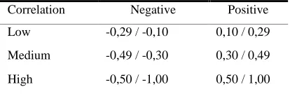
CC value varies between -1 and +1. A positive value of CC indicates that the two relationships are in the same direction. Negative values, on the other hand, indicate that the relationship is in the opposite direction. If the CC value is zero, it can be said that there is no relationship between two values. Detailed explanation for CC value is shown in Table 2, by Cohen [34].

Table 2. Cohen’s Correlation Table

Correlation Negative Positive

Low -0,29 / -0,10 0,10 / 0,29

Medium -0,49 / -0,30 0,30 / 0,49

High -0,50 / -1,00 0,50 / 1,00

4.2. Error Metric: Root Mean Square Error

Root Mean Squared Error (RMSE) is calculated by taking the square root of Mean Squared Error (MSE) value. MSE is a commonly used metric. Many mathematical techniques use MSE since it is the easiest metric to process. Its field of use in ML is to evaluate the performance of the classifiers [32].

Error rate of an estimator arises just because of an arbitrary estimation or lack of information that may provide an accurate estimation [35]. If the values of MSE and RMSE rates are closer to zero, the error rates will be lower. In addition, acceptable error values for MSE and RMSE are different for each learning problem.

MSE and RMSE calculations are shown below. Hereunder, p represents the estimated values and a represents the actual values.

𝑀𝑆𝐸= (𝑝1−𝑎1)2+⋯+(𝑝𝑛−𝑎𝑛)2

𝑛 (15) 𝑅𝑀𝑆𝐸= �(𝑝1−𝑎1)2+⋯+(𝑝𝑛−𝑎𝑛)2

𝑛 (16)

4.3. Bias Variance Decomposition

Bias-Variance decomposition is a key tool to understand ML algorithms. In recent years, the use of Bias-Variance decomposition in experimental studies is increasing gradually [32]. Bias and Variance concepts help to explain that very simple estimators are superior to complex ones and model collections are superior to simple models. In addition to statistical error functions, Bias-Variance decomposition is also derived for quadratic loss functions [36]. This derivation is shown in a study by German, Bienestock and Doursat [37]. In this notation the average error of learning algorithm is stated as the sum of the variance and the square of bias.

Having a as the actual value of a sample and p as the estimated value; the notation of average quadratic error as bias-variance decomposition is shown in the equation (17).

𝐸[(𝑝𝑖− 𝑎𝑖)2] =𝑉𝑎𝑟(𝑁𝑜𝑖𝑠𝑒) + 𝐵𝑖𝑎𝑠2+ 𝑉𝑎𝑟(𝑝𝑖) (17)

When the noise is omitted, the average quadratic error becomes the equation (18).

𝑀𝑆𝐸=𝑉𝑎𝑟𝑖𝑎𝑛𝑐𝑒(𝑝) + 𝐵𝑖𝑎𝑠2 ₍₁₈₎

4.4. k-Fold Cross Validation

Thus, the classifier is tested k times and trained. Classifier is trained on data set always with one less fold [15]. That is to say, k-1 from k sub-section is used for training. The remaining folds are used as test data [19]. Accuracy estimation of the classifier is average accuracy for k number multiple [15].

To make the most accurate estimation of error rate for common tests on various data sets using different learning techniques, the correct number is approximately 10. That is why k value is taken as 10 in this study. Theoretical evidences also support this situation [32].

k fold CV technique is a high cost technique in terms of calculations. However, it is very useful when we need to predict the error rate of the classifier [38]. Besides, k fold CV is also used to compare two different learning algorithms that have limited data [39]. Another important problem regarding k fold CV is the unbalance between the classes of the instances that are distributed to training and test sets [32]. Due to this unbalance, the classifier cannot perform a complete learning. For this reason, error rates of the classifier can be high. In order to solve this problem, each class should be evenly distributed between training and test sets. This ensures a solution for the problem. The process applied to solve this problem is called “stratifcation”. Stratification provides a precaution for unbalanced representation in training and test sets [32]. Weka implements stratification process while k fold CV technique and this produces reliable results [40].

Machine learning uses Leave-one-out cross-validation (LOOCV), which is the specific form of k fold CV method, while testing the performances of the classifiers. This method is also based on using only one observation instance from the original instance as validation data. That is to say, while one instance over original instances becomes validation instance, the others are used as training instances. This is repeated until all the instances used as validation instance. This method is particularly used to show how the models generated by classifiers are different from each other. If the models produce completely different results in each situation, then the original instances shoulde be revised, since these intances may be noised.

5. RESULTS AND DISCUSSION

All the experiments were done using the data with a number of 37308. Firstly, contribution of each feature to learning was calculated. In order to do

this, firstly, CC and RMSE values of feature set were compared by leaving out each feature once. Feature set with highest CC and lowest RMSE was selected as optimum feature set. In addition, if the left out features cause CC value to decrease dramatically, we can say that these features have an important contribution to learning. All the classifiers used in these experiments are adjusted according to default parameters. This process is called feature selection.

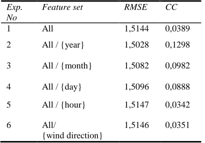
In Table 3, learning results of RBFNetwork classifier based on feature set is shown. According to these results, “hour” feature has a great contribution to learning, as CC value decreases dramatically and RMSE value increases remarkably. In addition, elimination of “year” feature leads to an increase in CC and a decrease in RMSE values compared to the first experiment. This may be because; RBFNetwork classifier did not learn the feature of “year” sufficient enough.

Table 3. Learning Results Of Rbfnetwork Classifier Based On Feature Set.

Exp. No

Feature set RMSE CC

1 All 1,5144 0,0389

2 All / {year} 1,5028 0,1298

3 All / {month} 1,5082 0,0982

4 All / {day} 1,5096 0,0888

5 All / {hour} 1,5147 0,0342

6 All/

{wind direction}

1,5146 0,0351

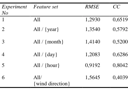
Table 4 Learning Results Of Knn Classifier Based On Feature Set.

Experiment No

Feature set RMSE CC

1 All 1,2930 0,6519

2 All / {year} 1,3540 0,5792

3 All / {month} 1,4140 0,5200

4 All / {day} 1,2083 0,6286

5 All / {hour} 0,9192 0,8042

6 All/

{wind direction}

1,5645 0,4039

Table 5 shows the learning results based on the feature set of Bagging classifier. According to these results, “wind direction” feature has a great contribution to learning as CC value decreases dramatically and RMSE value increases remarkably. In addition, elimination of “hour” feature leads to an increase in CC and a decrease in RMSE values compared to the first experiment. This may be because; Bagging classifier did not learn the feature of “year” sufficient enough.

Table 5. Learning Results Of Bagging Classifier Based On Feature Set.

Exp. No Feature set RMSE CC

1 All 0,8912 0,8089

2 All / {year} 1,0183 0,7411

3 All / {month} 1,1208 0,6743

4 All / {day} 1,0882 0,6967

5 All / {hour} 0,8845 0,8121

6 All/

{wind direction}

1,1429 0,6585

Table 4 shows the learning results based on the feature set of REPTree classifier. According to these results, “wind direction” feature has a great contribution to learning as CC value decreases dramatically and RMSE value increases remarkably. In addition, elimination of “hour” feature leads to an increase in CC and a decrease in RMSE values compared to the first experiment. This may be because; REPTree classifier did not learn the feature of “hour” sufficient enough. In addition, it is seen that only Bagging classifier that uses REPTree algorithm as base-classifier gives

good results compared to REPTree algorithm. This is because that Bagging is a successful method.

Table 6. Learning Results Of Reptree Classifier Based On Feature Set.

Experiment No

Feature set RMSE CC

1 All 0,9630 0,7757

2 All / {year} 1,0694 0,7123

3 All / {month} 1,1435 0,6601

4 All / {day} 1,1029 0,6875

5 All / {hour} 0,9376 0,7879

6 All /

{wind direction}

1,2501 0,5821

In Table 7, learning results of ZeroR classifier based on feature set is shown. According to these results, all the features have the same contribution to learning, since ZeroR is a majority-based classifier. Because of this, features do not have an important impact on CC and RMSE values. In addition, ZeroR classifier defines the base level of learning performances of digger classifiers. That is to say, no classifier may have lower performance than that of ZeroR classifier.

Table 7. Learning Results Of Zeror Classifier Based On Feature Set.

Exp. No Feature set RMSE CC

1 All 1,5156 -0,0115

2 All / {year} 1,5156 -0,0115

3 All / {month} 1,5156 -0,0115

4 All / {day} 1,5156 -0,0115

5 All / {hour} 1,5156 -0,0115

6 All/

{wind direction}

1,5156 -0,0115

“hour” feature increases the performance. In this case, when constituting the next experiment platform, we will consider the feature set with all the fetures but not “hour” feature. These two feature sets will be analysed by changing the parameters of the classifiers this time. Thus, the feature set and the classifier with best resuls will be tried to be determined. Accordingly, if we order the features from smaller to bigger, based on the amount of information they give about wind speed, we get the list of; {wind direction, month, day, year, hour}.

Table 8. Average Learning Results Of Al The Classifier Results.

Exp. No Feature set RMSE CC

1 All 1,1654 0,5689

2 All / {year} 1,2361 0,5406

3 All / {month} 1,2966 0,4882

4 All / {day} 1,2273 0,5254

5 All / {hour} 1,0640 0,6096

6 All/{wind direction} 1,3680 0,4199

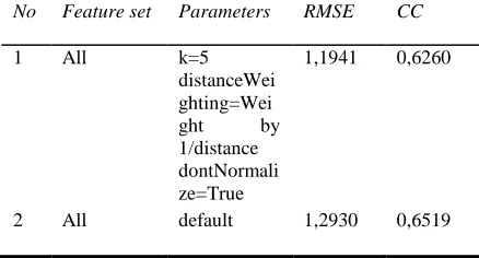
If the results in Table 9are analysed, it is seen that kNN classifier learns the feature set better when “hour” feature is left out. In addition, changes in kNN classifier’s parameters affect the result seriously. For the experiments 3 and 4, there is an increase of 0,0216 in CC value. However, a decrease of 0,0589 in RMSE value is observed. These values are important even they do not increase learning seriously. Nevertheless, the highest CC value is 0,8258.

Table 9. Learning Results Of Knn Classifier According To Parameter And Feature Set Changes.

No Feature set Parameters RMSE CC

1 All k=5 distanceWei ghting=Wei ght by 1/distance dontNormali ze=True

1,1941 0,6260

2 All default 1,2930 0,6519

3 All/ {hour} k=5 distanceWei ghting=Wei ght by 1/distance

dontNormali ze=True

0,8603 0,8258

4 All/ {hour} default 0,9192 0,8042

When the results in Table 10 are analysed, it seen that Bagging classifier learns better the feature set wit all the features. In addition, changes in Bagging classifier’s parameters do not seriously affect the results. CC value difference between experiments 1 and 3 is 0,0186. However, a decrease of 0,0373 is observed in RMSE values. These values are also important even they do not increase learning seriously. In addition, changes in parameters affect the performance of Bagging classifier. Especially two parameters remarkably affects the learning time of the classifier. However, there is no serious increase in test time. Besides, the important thing is that test time is lower than learning time. Yet, this is not the same for kNN classifier. For kNN classifier, test time is also long. That is because kNN classifier produces a local model rather than a general one. Local models always increase the test time. If training set has quite a number of instances, the performance of the classifier decreases. In addition, another superior feature of REPTree classifier over kNN classifier is that its model is clear. This kind of model always gives more information and produces comprehensible results for the observers of the model.

If we study the changed parameters of Bagging classifier, we see that firstly pruning of the tree that is produces by “noPruning” is selected. This change increases CC value. Pruning of the tree helps to overcome the errors caused by variance in the model. If an accurate estimation of test set is necessary, then pruning of the tree will be a good choice. The other parameter is called “numIterations”. The default value for this parameter is 10. An increase in this value leads to an increase in CC value. “numIterations” parameter represents the bag number of Bagging classifier.

For N=M, increasing M in equation (1-1/N)M≈ e

-1

reason, value of 0,368 should be lowered as much as possible. While doing this, M should have an optimal value so that the performance will not be reduced.

Consequently, the highest CC value is obtained by experiment 1 and CC value is 0,8275 and RMSE value is 0,8539 of experiment 1. However, this model causes some errors at the least arising form variance. For this reason, value of “noPruning” parameter shoulde be set as “False”. In addition, there is not a big difference between the values of experiments 1 and 2. Besides, there is not also a big difference between the values of experiments 5 and 2. As a result, conditions of the experiment 2 will be valid for test set as well.

Table 10. Learning Results Of Bagging Classifier Based On Parameter And Feature Set Changes.

No Feature set

Parameters RMSE CC

1 All numIterations=4 0

noPruning=True

0,8539 0,8275

2 All numIterations=4 0

0,8774 0,8154

3 All default 0,8912 0,8089

4 All/ {hour}

numIterations=4 0

noPruning=True

0,8741 0,8190

5 All/ {hour}

numIterations=4 0

0,8772 0,8155

6 All/ {hour}

default 0,8845 0,8121

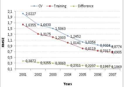
In Table 11, performance results of Bagging classifiers that gives the highest CC and lowest RMSE values are shown in terms of training sets prepared according to years. Performed test are two kinds as 10 fold cross-validation and training data only. So, the bias – variance balance can be observed for model produced by the classifier. The results obtained by cross-validation are Error RateCV and Correlation CoefficientCV values.

Performance result of the classifier, when all the data set is used as training set, is Error RateTraining

and Correlation CoefficientTraining. The important

value here to measure bias-variance balance is the comparison of Error RateCV and Correlation

CoefficientCV values. While number of training data

is rising, the difference between ErrorRateTraining

and ErrorRateCV is considered. If this difference is

high and ErrorRateCV is also high, then it can be

said that there is high varience in the model. If the difference between ErrorRateTraining and

ErrorRateCV is low and ErrorRateCV value is high,

then it can be said that the classifier has a high variance.

Table 11. Performance Results Of Bagging Classifier On Training Sets That Are Prepared According To Years

No Years Number

of Data

RMSECV CCCV

RMSETraining CCTraining

1 2001 2570 2,0227 0,7686 1,6355 0,8579 2 2001-2002 5324 1,6430 0,8043 1,3175 0,8821 3 2001-2003 7379 1,5063 0,8107 1,2003 0,8872 4 2001- 2004 11569 1,2452 0,8117 1,0141 0,8826 5 2001-2005 20292 1,0356 0,8106 0,8119 0,8914 6 2001-2006 29025 0,9304 0,8214 0,7317 0,8967 7 2001-2007 37308 0,8774 0,8154 0,6905 0,8932

When the results in Fig.1 are analyzed, it is seen that the difference between the starting values of RMSECV and RMSETraining is not very high.

However, as the number of training data increases over the years, the difference between RMSE values slowly decreases as well. As a result of this, errors caused by high variance are observed. In addition, it can be said that the model produced by Bagging classifier may cause high error rates because of high RMSECV value between the years

2001 and 2007. The difference between RMSECV

and RMSETraining for the data in 2001 is 0,3872,

however, when the data set between 2001 and 2007 is used, the difference decreases to 0,1869. Increasing the number of training data is one of the ways to overcome the errors caused by high variance. Using a compound feature or making normalization over the data are also alternative solutions.

Fig. 2 shows the comparison between the real wind speed values and the wind speed values estimated by Bagging classifier. The size of “X” signs in the figure shows the size of errors of the classifier. Small “X” signs in the figure show that the errors done by the classifier are also small. In other words, as the errors rise in numbers, the sign grows bigger, and as the errors decrease in numbers, the sign becomes smaller. According to this information, the estimations made are mainly correct. The estimations which have a big sign are less in common, and they consist of estimations which have a big difference between the real value and the estimated value. This situation shows that there is a very chaotic weather situation in that example, and it is verified with the high correlation coefficient value of 0,8154.

Figure 2. The Comparison Of Actual Wind Speed Values (X-Axis) And Predicted Wind Speed Values (Y-Axis)

In Table 12, performance results of Bagging classifier whose parameters are set for the best results, according to “k” value. In most studies, it is theoritacally explained that “k” should have the value of 10. Besides, in most studies as well “k” value is set as 10 or set according to LOOCV method. In this study, “k” value is assumed as 10 in every experiment. In Table 12, it is clearly seen how changes in “k” value affects the performance. According to this, it is understood that “k” value does not affect the learning result of the classifier.

Table 12. Performance Results Of Bagging Classifier According To “K” Value.

No k-Fold Value

RMSE CC

1 2 0,9536 0,7772

2 5 0,8946 0,8072 3 10 0,8774 0,8154

4 20 0,8680 0,8199

5 30 0,8690 0,8193

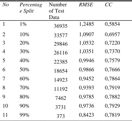
In Table 13, performance results are shown by using a specific percent of learning set as training set and the remaining part as test set with Bagging classifier. In experiment 1, %1 of learning set is used as training set and the remaining %99 is used as test set. Accordingly, CC value is assessed as 0,5854 and RMSE value is assessed as 1,2485. With an increase in training set, CC value increases but RMSE value decreases. This results show that in worst case CC value does not drop below 0,5. In addition, if CC value is higher than 0,5, then this shows that the correlation between actual and predicted values is high.

Table 13. Performance Results By Using A Specific Percent Of Learning Set As Training Set And The Remaining Part As Test Set With Bagging Classifier.

No Percentag e Split

Number of Test Data

RMSE CC

1 1% ₃₆₉₃₅ 1,2485 0,5854

2 10% 33577 1,0907 0,6957

3 20% 29846 1,0532 0,7220

4 30% ₂₆₁₁₆ 1,0351 0,7370

5 40% ₂₂₃₈₅ 0,9946 0,7579

6 50% ₁₈₆₅₄ 0,9866 0,7666

7 60% ₁₄₉₂₃ 0,9452 0,7864

8 70% ₁₁₁₉₂ 0,9393 0,7919

9 80% ₇₄₆₂ 0,9785 0,7882

10 90% ₃₇₃₁ 0,9736 0,7929

11 99% ₃₇₃ 0,8423 0,7819

In Fig.3 the correlation graph between the actual values and predicted values of Bagging classifiers about January, 2010 is shown. When the graph is analyzed, it is seen that the variance between actual and predicted values is very high on 24th January. Apart from that, the predictions are close to actual values. This shows that Bagging classifier produces good results and can be used for wind speed predictions.

Fig. 4 shows the monthly average values of wind speed estimations made by Bagging classifier in 2013. According to the figure, the first three months have a higher speed rating than the other months. According to the estimations, the month with the least wind speed is December.

Figure 4. Average Wind Speed Forecasts For Year 2013

6. CONCLUSION

In this study, the wind potential of Kırklareli, a city located in the west of Turkey is analyzed, and the data between the years of 2001-2007 is used. The predictions about the year 2010’s wind speed calculations are made according to this training data. Also, with the application of cross validation method on the training data, the correlation coefficient value between the real values and the predicted values are obtained as 0,8154. The machine learning classifier which is able to obtain such a high correlation value is the Bagging classifier using REPTree classifier as a base-learner. Also, five input attributes are chosen to be used in the training sets. These attributes are year, month, day, hour and the wind direction. Among these attributes, the wind direction attribute significantly enhances the success rate of the predictions of Bagging method and REPTree classifier. As a result of all these applications, the Bagging classifier is found very successful as a machine learning classifier and as a method of choosing attribute.

REFERENCES

[1]. WWEA (2009) World Wind Energy Report 2008.

http://www.wwindea.org/home/images/stories/ worldwindenergyreport2008_s.pdf. Accessed 19 February 2013.

[2]. WWEA (2012) 2012 Half year Report. http://www.wwindea.org/webimages/Half year_report_2012.pdf. Accessed 19 February 2013.

[3]. Etemoglu AB, İsman MK (2004) Enerji Kullanımının Teknik ve Ekonomik Analizi. Mühendis ve Makina, 45(529):19 23

[4]. TUİK (2012) Nüfus Projeksiyonları, 2013-2075.

http://www.tuik.gov.tr/PreHaberBultenleri.do?i d=15844. Accessed 17 November 2012.

[5]. Güler O (2005) Dünyada ve Türkiye’ de Rüzgâr Enerjisi. V. Enerji Sempozyumu, 161-167, Ankara, Turkey

[6]. TMMOB (2012) Türkiyenin Enerji Görünümü. http://www.mmo.org.tr/resimler/dosya_ekler/d d924b618b4d692_ek.pdf. Accessed 19 February 2013.

[7]. TWEA (2012) Turkish Wind Energy Statistics Report.

http://tureb.com.tr/attachments/article/168/Tur kiye%20Ruzgar%20Enerjisi%20Istatistik%20

Raporu%202012-Turkish%20W%C4%B1nd%20Energy%20Stat istics%20Report%202012.pdf. Accessed 19 February 2013.

[8]. İlkılıç C (2009) Türkiye’de Rüzgar Enerjisi Potansiyeli ve Kullanımı. Mühendis ve Makina, 50(593):26-32

[9]. Ersoz S, Akinci TC, Nogay HS, Dogan G (2012) Determination of wind energy potential in Kirklareli-Turkey. International of Green

Energy- Taylor & Franchis.

doi: 10.1080/15435075.2011.641702

[10].Gokcek M, Bayulken A, Bekdemır S (2007) Investigation of wind characteristics and wind energy potential in Kirklareli, Turkey. Renew Energy, 32(10):1739-1752

[11].Erdil A, Arcaklioglu E (2012) The prediction of meteorological variables using artificial neural network. Neural Computing and Applications. doi: 10.1007/s00521-012-1210-0 [12].Hocaoglu FO, Oysal Y, Kurban M (2009)

Missing wind data forecasting with adaptive neuro-fuzzy inference system. Neural Computing and Applications 18(3):207–212 [13].Herva´s-Martı´nez C, Salcedo-Sanz S,

Gutie´rrez PA, Ortiz-Garcı´a EG, Prieto L (2012) Evolutionary product unit neural networks for short-term wind speed forecasting in wind farms. Neural Computing and Applications 21(5):993–1005

[14].Samuel AL (1959) Some studies in machine learning using the game of checkers. IBM J. Res. Devel. 3:210-229

[16].Duda RO, Hart PE, Stork DG (2001) Pattern classification - 2nd ed., New York, Wiley-Interscience.

[17].Amasyalı MF (2008) Yeni Makine Öğrenmesi Metotları ve İlaç Tasarımına Uygulamaları. Thesis (Phd). Yıldız of Technical University. [18].Breiman L (1996) Bagging Predictors.

Machine Learning, 24:123–140

[19].Alpaydın E (2004) Introduction to Machine Learning. The MIT Press, Printed and bound in the United States of America. ISBN: 0-262-01211-1

[20].Efron B, Tibshirani R (1993) An Introduction to the Bootstrap. Boca Raton, FL: Chapman & Hall/CRC.

[21].Yakupoglu C, Atıl H (2006) A Study on Bootstrap Method and It’s Application II. Confidence Interval, Hypothesis Testing and Regression Analysis with Bootstrap Method, Ege Üniv. Ziraat Fak. Dergisi, 43(2):63-72, ISSN 1018-8851

[22].WEKA,

http://weka.sourceforge.net/doc/weka/classifier s/trees/REPTree.html. Accessed 25 December 2012.

[23].Beyer K, Goldstein J, Ramakrishnan R, Shaft U (1999) When Is `Nearest Neighbor' Meaningful?. Proceedings of the 7th International Conference on Database Theory, 217-235

[24].Kocamaz AF, Aydın F, Ucar E (2011) Developing of a learning-based system to assist treatment process of arrhythmia patients. Scientific Research and Essays, 6(32):6654-6665

[25].Manning CD, Raghavan P, Schütze H (2008) Introduction to Information Retrieval.

Cambridge University Press, ISBN: 0521865719

[26].Moody J (1989) Fast learning in networks of locally-tuned processing units. Neural Computation, 1: 281-294

[27].Casdagli M (1989) Nonlinear prediction of chaotic time series. Physica D, 35: 335 356 [28].Broomhead DS, Lowe D (1988) Multivariable

functional interpolation and adaptive Networks. Complex Systems, 2:321-355

[29].Matej S, Lewitt RM (1996) Practical considerations for 3D image reconstruction using spherically volume elements. IEEE Trans. On Medical Imaging, 15:68-78

[30].Mashor MY (2000) Hybrid Training Algorithm for RBF Network. In International Journal of the Computer, The Internet and Management, 50-65

[31].Zhang JG, Deng HW (2007) Gene selection for classification of microarray data based on the Bayes error. BMC Bioinformatics, 8:370 [32].Witten IH, Frank E (2005) Data mining:

practical machine learning tools and techniques – 2nd ed.. the United States of America, Morgan Kaufmann series in data management systems.

[33].Stigler SM (1989) Francis Galton's Account of the Invention of Correlation. Statistical Science 4(2):73-79

[34].Cohen J (1988) Statistical power analysis for the behavioral sciences (2nd ed.). Hillsdale, NJ: Lawrence Erlbaum Associates.

[35].Lehmann EL, Casella G (1998) Theory of Point Estimation (2nd ed.). New York: Springer. ISBN 0-387-98502-6.

[36].Domingos P (2000) A Unifed Bias-Variance Decomposition and its Applications. In Proc. 17th International Conf. on Machine Learning, 231-238

[37].Geman S, Bienenstock E, Doursat R (1992) Neural networks and the bias/variance dilemma. Neural Computation, 4(1):1-58

[38].Nilsson NJ (1996) Introduction to Machine Learning: An Early Draft of a Proposed Textbook, Robotics Laboratory, Department of Computer Science, Stanford University. [39].Mitchell TM (1997) Machine Learning,

McGraw-Hill Science/Engineering/Math, ISBN: 0070428077, pp. 432.

[40].Bouckaert RR, Frank E, Hall M, Kirkby R, Reutemann P, Seewald A, Seuse D (2008) WEKA Manual for 3.6.0, http://prdownloads.sourceforge.net/weka/Weka Manual-3.6.0.pdf?download. [Access: 24 June 2011].