MULTI LEVEL GROUP KEY MANAGEMENT TECHNIQUE FOR MULTICAST SECURITY IN MANET

ALGORITHM FOR REDUNDANT NODES DEPLOYMENT OF

GREENHOUSE WSN MONITORING AND CONTROL

SYSTEM

ZHANG LEI

Department of Electrical & Electronic Engineering, Henan University of Urban Construction, Ping Ding Shan, 467036, China

E-mail: [email protected]

ABSTRACT

Specific to the funneling effect of Greenhouse wireless sensor networks (WSN) monitoring and control system, redundant nodes deployment algorithm (RNDA) is proposed. RNDA deploys a certain number of redundant nodes based on load of nodes so as to balance energy consumption of network. By means of introducing the next-hop routing probability of node into graph theory as the weight, the probability theorem that source node data arrive at the destination node after making m hop(s), thus providing an effective for researching network data transmission. Theoretical analysis and simulation result show that while remarkably extending network life, RNDA can also effectively balance energy consumption of network nodes.

Keywords: Wireless Sensor Networks (WSN), Greenhouse Monitoring And Control System, Redundant Nodes Deploy, Funneling Effect, Graph Theory

1. INTRODUCTION

WSN (wireless sensor networks) boasts low cost, low energy consumption, flexible networking, no need for wiring and other advantages. Combination of WSN and greenhouse monitoring and control system is an urgent need of modern agricultural production. In a greenhouse WSN monitoring and control system, a large number of sensor nodes are deployed in a dense way, featuring a considerable number of redundant nodes. In WSN monitoring and control system based on centralized data acquisition, data are mostly transmitted to base station by way of multi-hop. Nodes close to base station die out too soon due to transmission of large volumes of data, resulting in division or even total paralysis of the network. Such energy consumption phenomenon caused by imbalanced load of nodes is called funneling effect [1-2].

Node redundancy technology is extensively used for improving performance of WSN. Zhang Zhenjiang et al. combine some redundant nodes in WSN into a trunk to serve as an agent for information transmission in the network, thus saving normal nodes and cluster head energy [3]; Chen Feng et al. meet coverage of 3D monitoring area by awakening redundant sleeping nodes by stages [4]. These approaches use existing redundant nodes in the network to extend network life and meet network coverage; but they fail to take into

consideration the issue of redundant nodes deployment.

Graph theory is often used for describing relationship and connectivity between nodes, serving as a useful mathematic tool for the research on network structure [5]. Presently, in terms of acquisition shortest network path [6-7], strongest

connectivity path, network evaluation/optimization [8] and so on, an array of

application researches has been made with graph theory. This article, taking greenhouse WSN as the application background and based on relevant graph theory, proposes the theorem of arrival rate of data following m hop(s) in network, and designs the Redundant Nodes Deployment Algorithm (RNDA) based on balanced load. Theoretical analysis and simulation result show that RNDA remarkably extends network life and also effectively solve funneling effect of greenhouse WSN monitoring and control system.

2. ISSUE DESCRIPTION

deployment is acquisition of load of each node against diversified network layout. In this article, the issue is introduced with the example of 2D-layout greenhouse WSN monitoring and control system in greenhouse environment. By way of model building for analysis, eventually a scheme on redundant nodes deployment applicable to any layout is obtained.

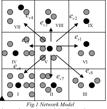
[image:2.612.113.286.359.535.2]

Suppose the greenhouse is rectangular, on the condition of meeting area coverage and ensuring connectivity between all adjacent grids, and with sensor node sensing distance and wireless communication distance taken into account, the monitoring area is divided into several virtual grids. At any time, only one node in the grid is active while other nodes are redundant nodes configured according to energy consumption of each grid. The network submits monitoring data to the base station by way of multi-hop. Nodes in the virtual network awake to operate within their own active period as per order specified in advance. With the end of operation in this period, the node will immediately enter sleep status.

Fig.1 Network Model

Fig. 1 shows the model of greenhouse WSN monitoring and control system network, where the black nodes are active nodes, grey ones are redundant ones, each grid is coded with Roman numerals, and arrows show routing direction of nodes.

Definition 1: The probability in which Node

v

selects Edge

e

as the routing of next hop is called Node

v

's

e

direction routing probability, expressed as

P

v

(

e

)

. If

P

v

(

e

)

=0, this direction can not be

used for communication.

Definition 2: Node

v

, in the direction of

n

presents a routing probability set{

P

v

(

e

v1

)

,

P

v

(

e

v2

)

,…,

P

v

(

e

vn

)

}, this set is

called routing probability vector of Node

v

, briefly called probability vector of

v

, expressed as

P

_v.

3. RADA

3.1 Calculation of Load Distribution

In the greenhouse, the network topology of active nodes can be expressed as Graph

>

=<

V

R

G

,

. In the figure,

V

=

{

v

₁

,

v

₂

,...,

v

_n

}

is the node set of graph, Element

v

_i is node of graph,

R

=

{

e

₁

,

e

₂

,...,

e

_n

}

is edge set of the graph, its Element

e

_i

=

{

<

v

_j

,

v

_k

>

|

1

≤

j

≤

n

,

1

≤

k

≤

n

}

is the

edge of the graph,

v

_j is the starting point of

e

_i,

k

v

is the end point of

e

_i, and routing probability

)

(

_i

v

e

P

=

R

( )

v

_j

,

v

_k

=

r

_jk

∈

[

0

,

1

]

is the weight of Edge

i

e

.

n

order square matrix

n n jk

G

r

R

=

(

)

_× is called as

G

's adjacency matrix, where

r

_jk

=

R

(

v

_j

,

v

_k

)

,

it is specified that when

j

=

k

,

r

jk

=

0

.

According to the basic graph theory theorem [9] provided in Bibliography, the following source-node to destination-source-node m hop(s) data arrival rate theorem can be obtained.

Theorem: Suppose in directed graph

>

=<

V

R

G

,

,

V

=

{

v

1

,

v

2

,...,

v

n

}

,

n n jk

G

r

R

=

(

)

_× is adjacency matrix of

G

,

n n m jk m

G

r

R

=

(

( )

)

_× , so

r

_jk(m) is the probability for Node

v

_j to make exactly m hop(s) to arrive at

v

_k.

Prove:

（1） When m=1, obviously it is tenable.

（2） Suppose when m=i, the theorem is tenable.

（3） When m=i+1, the theorem is tenable. Proved as follows:

n n n

p i pk jp i

G G i G n n i

jk

R

R

R

r

r

r

× =

+ × +













⋅

=

⋅

=

=

∑

1 ) ( 1

) 1 (

)

(

i.e.

∑

=

+

₌

n

_⋅

p

i pk jp i

jk

r

r

r

1 ) ( 1

In this formula,

r

_jp shows the probability for

Node

v

_j to make 1 hop to reach

v

_p,

r

_pk(i) is the probability for Node

v

_p to make

i

hop(s) to reach

k

v

. So

r

_jp

⋅

r

_pk(i) is the reachable probability for

starting from Node

v

_j, passing

v

_p and arriving at

1 v

e

2 v

e

3

v

e

4 v

e

5 v

e

6 v

e

7 v

e

e

v8

I II III

IV V VI

IX VIII

k

v

while the total hop number is i+1;

therefore,

∑

=

⋅

n p i pk jp

r

r

1 ) (

is the probability for starting

from Node

v

_j and making i+1 hops to arrive at

k

v

.Over.

Based on the above-mentioned theorem, it is possible to obtain the data load volume of any Node

i

v

. Suppose for a pair of nodes in the network, data can go from one to the other node within m hop(s), the arrival rate matrix sequence within m hop(s)｛

1 G

R

,

R

_G2, ……,

R

_Gm｝ is obtained. Sum of Matrix

∑

= m k k G

R

1

's Column

i

,

∑∑

= = n j m k k ji

r

1 1

, is the probability

sum for each node to make 1 to m hop(s) to arrive at

v

_i . Therefore,

v

_i receiving and transmission loads are respectively,

∑∑

= =

⋅

=

n j m k k ji

Rv

l

r

D

i 1 1 (1)

∑∑

= =

+

=

n j m k k ji

Tv

l

r

D

i

1 1

)

1

(

(2)

In this formula,

l

is the data volume generated by each node for finishing the monitoring task, and

n

is the number of nodes.

3.2 Identification of subsections

In a WSN, energy is mainly consumed for wireless communication. Energy consumed for sensing data, processing data and so on can be ignored. During wireless communication, power attenuation of transmission signals presents an exponential decay along with increase in transmission distance. In this article, free space and multi-path attenuation model proposed in Bibliography [10] is used.









×

×

+

×

×

×

+

×

=

₄ 2

d

l

E

l

d

l

E

l

E

amp elec fs elec TX

_ε

ε

0 0

d

d

d

d

≥

<

(3) elec

RX

l

E

E

=

×

(4) In the formula,

d

is communication distance;

l

is transmission or receiving data bit;

d

₀is the critical value for switching between the two models;

E

_elec is the energy consumption for transmitting (or receiving) 1 bit data during operation of transmission/receiving circuit;

ε

_fsand

amp

ε

respectively are energy consumption for power amplification under the two models. For easy calculation, it is supposed herein:

d

<

d

₀.

According to Node

i

's data receiving volume

i

Rv

D

and data transmission volume

i

Tv

D

obtained based on Formulas (1) and (2), the below periodical energy consumption of Node

v

_i can be obtained based on Formulas (3) and (4)

2

)

(

D

D

E

D

d

E

_{i Rv Tv elec Tv fs}

i i

i

+

⋅

+

⋅

⋅

=

ε

(5)

3.3 Node Deployment

Suppose each node comes with the same initial energy

E

_ini and the node can not work properly if falling below the same energy threshold; in ideal status, it is expected that all virtual grids come with the same life, i.e.:

1 1

)

1

(

)

1

(

+ +

+

=

+

i ini i i ini i

E

E

b

E

E

b

1

1

≤

i

≤

n

−

(6)

Organized into: 1 1 1 1 + + + +

−

+

×

=

i i i i i i i

E

E

E

b

E

E

b

(7)

This formula is an n term linear equation, by selection of specific node to be configured with certain redundant node number as initial condition, the number of redundant nodes needed for other nodes can be obtained. We can configure any number of redundant node(s) for Grid I as the initial condition.

4. SIMULATION ANALYSIS AND RESULT

The analysis shows that the key of the above algorithm lies in determination of probability vector

v

[image:4.612.78.295.107.309.2]

Table 1 Table of Probability Vectors

Table 2 Table of Simulation Parameters

Parameter Value Parameter Value Area 100m

×

10

0m

Active node number a 5 Each node

Data volume

k

256 bit Eelec 50nJ/bit

Node initial Energy Einit

2J

ε

fs 10pJ/bit/m2

Energy lower limit

Einit

×

1%

ε

amp

0.0013pJ/bit/ m4 Data fusion

Coefficient

δ

1/a or 1 d0 86.2m

The simulation takes into consideration the influence on network life exerted by cluster head adoption of data fusion strategy and absence of this strategy. WSN data fusion mainly aims to reduce data volume of the network by integrating redundant information of all sensor nodes. In this simulation experiment, data fusion is carried out at cluster heads; when data fusion strategy is not used, data fusion coefficient is set to be

σ

=

1

; when the strategy is used, different data fusion coefficient can be selected based on varied fusion degree. As sensor nodes here are all isometric sensor nodes, information collected by them is of the same type. According to statistical knowledge, environment parameters in a small scope differ little. Therefore, data of all sub-nodes in a grid can be used into one datum to describe environment information in this grid (such as temperature and humidity). In simulation experiment, data fusion coefficient is set to be

σ

=

1/

a

when data fusion strategy is

adopted, where

a

is the number of active nodes in the grid. In all the simulation experiments below, it is set as 5.

In MATLAB 7.0, compile M document program to research performance of RNDA, and then make comparison with the pattern of even deployment. In the even deployment pattern, redundant nodes are evenly deployed to each cluster and the network still runs based on 3 task time slots. Below is the comparison of influence on network life exerted by the two patterns with varied grid number and fusion coefficient. Network life is defined as operation cycles when all hot clusters die.

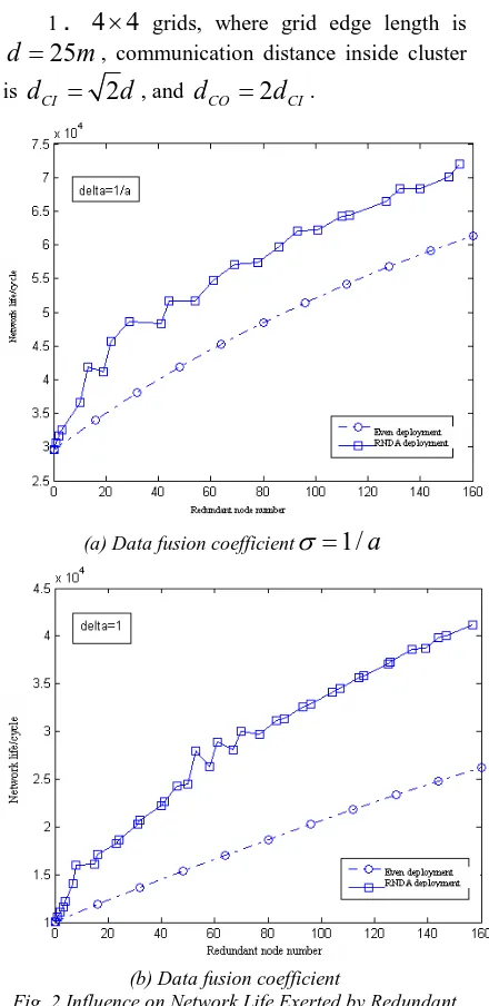
1．

4 4

×

grids, where grid edge length is

25

d

=

m

, communication distance inside cluster is

d

CI

=

2

d

, and

d

CO

=

2

d

CI.

(a) Data fusion coefficient

σ

=

1/

a

[image:4.612.312.532.253.705.2]

(b) Data fusion coefficient

Fig. 2 Influence on Network Life Exerted by Redundant

Nodes (

4 4

×

Grids)

Cluster head category

Routing Probability Vector

p

_v

Value range South border

cluster head

4 5

( ) ( )

{0,0,0, , ,0,0,0}

v v

v v e v e

p = p p (0,0,0,1/2, 1/2,0,0,0) West border

cluster head

7 8

( ) ( )

{0,0,0,0,0,0, _v , _v

v v e v e

p = p p (0,0,0,0,0, 0,1/2,1/2) General cluster

head

5 6 7

( ) ( ) ( )

{0,0,0,0, _v , _v , _v ,0

v v e v e v e

p= p p p (0,0,0,0,1/

3,1/3,1/3,0 )

East hot cluster head

5

( )

{0, 0, 0, 0, , 0, 0, 0}

v

v v e

p = p (0,0,0,0,1, 0,0,0) North hot

cluster head

7

( )

{0, 0, 0, 0, 0, 0, , 0} v

v v e

p = p (0,0,0,0,0, 0,1,0) Northeast hot

cluster head

6

( )

{0, 0, 0, 0, 0, , 0, 0

v

v v e

2 ．

5 5

×

grids, grid edge length being

d

=

20

m

.

(a) Data fusion coefficient

σ

=

1/

a

(b) Data fusion coefficient

σ

=

1

Fig. 3 Influence on Network Life Exerted by Redundant

Nodes (

5 5

×

Grids)

In Fig. 2 and Fig. 3, each discrete point on the curve stands for one simulation; their horizontal coordinate is the sum of redundant nodes of each cluster in this simulation; in the even deployment pattern, its value equals grid number

×

redundant node number which added to each grid; vertical coordinate of each simulation point stands for network life of this simulation.

In the first simulation, both even deployment pattern and RNDA deployment pattern come without redundant nodes; this is the initial status for both patterns, so the two curves meet here. An additional redundant node is added to each grid

with every simulation made in the even deployment pattern. On the other hand, in RNDA deployment pattern, as the northeast hot cluster head consumes the most energy, one redundant node is added to this cluster with each simulation. So given this initial condition, the redundant node number of other clusters are obtained according to calculation formula for redundant nodes.

Data fusion coefficient exerts a remarkable influence on network life. This is because when data fusion strategy is not used, network number is 5 times of that used when data fusion strategy is adopted. It can be seen from the figure that when data fusion strategy is adopted, network life is about 2-3 times that of the life when the strategy is not used.

Likewise, virtual grid number influences network life. The more grids divided in the monitoring area and the greater the data volume of the network, the shorter the network life is.

The comparison between the two redundant nodes deployment algorithms shows that when the same redundant nodes are deployed, RNDA enables a longer network life.

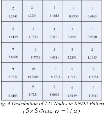
[image:5.612.331.506.439.633.2]

In Fig. 3(a), 125 redundant nodes are deployed on Points A and B on the curve. In even deployment pattern (i.e. Point A), 5 redundant nodes are deployed in each grid, while in RNDA deployment pattern, distribution of redundant nodes (i.e. Point B) are shown in Fig. 4.

Fig. 4 Distribution of 125 Nodes in RNDA Pattern

(

5 5

×

Grids,

σ

=

1/

a

)

relatively small variation to RNDA deployment curve, i.e. life of network with more nodes may fall shorter than network with less nodes. Such is relatively remarkable in Fig. 2(b). However, such case only occurs between two neighboring simulation points.

Moreover, as symmetrical routing probability vector is used, distribution of redundant nodes is symmetrical to the monitoring area against a 45-degree diagonal. The initial condition is set to be redundant node number of northeast hot cluster as with such a routing strategy, this cluster is the most energy-consuming one among the three hot clusters. At Point B, 19 redundant nodes join this cluster, showing that this is the 19th simulation experiment.

By comparison between network performance at Points A and B in Fig. 3(a), one can see RNDA extends network life by 35.8% in comparison with even deployment pattern. To extend the same network life, RNDA uses much less redundant nodes. When network life is

3

.

5

×

10

4 cycles, RNDA only deploys 24% of redundant nodes in the even pattern.

5. EQUATIONS

With greenhouse WSN monitoring and control system as application purpose, this article proposes redundant node deployment algorithm RNDA based on balanced load. This algorithm is closely related to routing; based on routing probability of nodes, this algorithm can be applicable to networks with multi dimensions and multi-path routing. With the next-hop routing probability of the node as edge weight, the theorem of m hop(s) arrival rate is proposed, thus providing a valid approach for researching on network data transmission. The simulation result shows that the algorithm well solves the funneling effect. By deploying of the same redundant nodes, RNDA enables longer network life. Given 125 redundant nodes are deployed, RNDA patterns extends the life by 35.8% in comparison with even pattern. For extension of the same network life, RNDA serve to save a large number of redundant nodes. When network life is

4

10

5

.

3

×

cycles, RNDA only deploys 24% of redundant nodes in the even pattern.

REFRENCES:

[1] Wan C Y, Eisenman S B, Campbell A T, et al. “Overload traffic management for sensor networks”. ACM Transactions on Sensor Networks, 2007, 3,Article No. 18．

[2] Ahn G S, Miluzzo E, Campbell A T, et al. “Funneling-MAC: A Localized, Sink-Oriented MAC For Boosting Fidelity in Sensor Networks”. In: Proceedings of the 4th international conference on Embedded networked sensor systems. New York: ACM, 2006, 293-306.

[3] Zhang ZJ, Liu Y. “An energy-efficient redundant nodes tree mechanism for wireless sensor networks”. In: Second International Conference on Systems and Networks Communications. Institute of Electrical and Electronics Engineers Computer Society , 2006, 63 – 63.

[4] Chen F, Jiang P, He Q. “Phased waking coverage scheme based on hibernation of redundant nodes for wireless sensor networks”. Proceedings-International Symposium on Computer Science and Computational Technology. NJ: Institute of Electrical and Electronics Engineers Computer Society, 2008: 709-713.

[5]Rickard J T, Yager R R. “Hypercube Graph Representations and Fuzzy Measures of Graph Properties”. IEEE Transactions on Fuzzy Systems, 2007, 15: 1278-1293.

[6] Cornelis C, Kesel PD, Kerre EE. “Shortest Paths in Fuzzy Weighted Graphs”. International Journal of Intelligent Systems, 2004, 19: 1051-1068.

[7] Boulmakoul A. “Fuzzy graphs modelling for HazMat telegeomonitoring”. European Journal of Operational Research, 2006, 175: 1514-1525.

[8] LászlóT. Kóczy. “Fuzzy graphs in the evaluation and optimization of networks”. Fuzzy Sets and Systems, 1992,46: 307-319. [9] Fu Yan, Gu Xiao-feng, “Wang Qing-xian, et al.

Discrete Mathematics and Its Applications”, Beijing: China Higher Education Press, 2007: 257-258.