Three Phase Fault Algorithm in Distribution System
by Using Database Approach and Impedance Based
Method
N.H.Shamsudin, A.Abdul Latiff, N.Abas Faculty of Electrical Engineering Faculty of Electronics and Computer Engineering
Universiti Teknikal Malaysia Melaka Durian Tunggal, Melaka, Malaysia
H.Mokhlis, L.J.Awalin Department of Electrical Engineering
Faculty of Engineering University of Malaya 50603, Kuala Lumpur
Abstract—A three phase fault location algorithm using database and impedance based method is utilized in distribution system to locate fault which may occur in any possible fault sections and to optimize the switching operations to reduce the outage time affected by fault. The configuration of 132/11kV from actual distribution system in Malaysia with 38 nodes is modelled using the PSCAD/EMTDC software. This work attempt to combine fault section identification with impedance based method in order to address non-homogeneity of cables in distribution system. The result which is the fault location result is obtained through the complete process which involves the database formation acquired through the PSCAD/EMTDC software simulator and the fault location distance calculation carried out by the MATLAB software. The comparison is made through proposed algorithm with actual data acquired from the utility board. Final outcome of the proposed algorithm shows good approximation on fault location.
Keywords-three phase fault location algorithm, distribution system, database formation, distances calculation.
I.INTRODUCTION
Electrical distribution system is an important infrastructure which highly contributes to Malaysia economic growth. Therefore any abnormal connectivity in distribution system can lead to a major disaster. Fault in distribution system can accidentally or intentionally occurs when distribution system having relatively low impedance between two points of different potential. Whenever fault occurs, high initial fault current will flow through the fault path resulting voltage drop along the power grid system. High fault current can damage transformer and cables in the power system and that can caused power failure on affected feeder. It means that the system should be well protected to ensure the reliability and quality of the power supply, leading to power interruption such as outage and voltage sag events. Such problems could be minimised by locating fault as fast as possible so that repair works and restoration of the faulty network can be done quickly. A fast fault location is also very important in distribution systems because the faults in the distribution
system affect a large number of customers. This is due to the fact that distribution systems are operated in radial configuration and are often fed by a single supply. When a fault occurs at any location along the feeder or at the laterals of the feeder, the circuit breaker at the main feeder operates to disconnect the main feeder from the source. Hence, customers along the main feeder or at the laterals connected to the feeder will experience a power outage.
Various methods of fault location have been used by utilities. Generally, the method can be divided into 3 categories, which are travelling wave [1], knowledge-based and impedance-based. Travelling wave method offers high accuracy, however higher cost is required due to complicated and expensive equipment such as Global Positioning System (GPS) and high-speed data acquisition device used for the installation [2]. For knowledge-based method, large consumption of time is used in the training process that necessarily repeated when the systems are changes. In impedance-based method, the acquisition of rms current and voltage with lumped model parameters is utilized to locate fault location accurately. Instead of other methods, this method contributes to major advantage of simplicity, accuracy and economic implementation.
A few restrictions should be taken into account mainly on fault resistance, fault location, source impedances, and the line and load modelling [3, 4]. Nevertheless, the natures of its significant dependence on a configuration of distribution system and model parameters lead to problem for method used [4].
This paper is organized as follows. In section II, the modelled distribution network is tested by using commercial available simulation software. Section III discusses on how the hybrid method is constructed. Analysis of simulation results and conclusion are discussed in section IV and V respectively.
II.TEST SYSTEM MODELLING
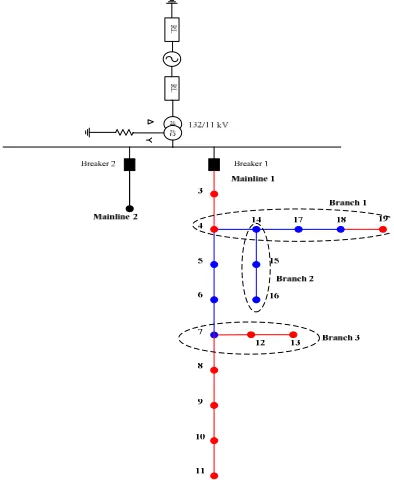
the test system in PSCAD/EMTDC simulation software, the three phase fault algorithm is implemented in MATLAB programming. The one line diagram of the tested network is shown in Fig. 1. For generating results from simulation, three phase fault with zero fault impedance is firstly created on nodes and lines. From that, the value of harmonic components of inflow current and voltage through the circuit breaker during fault occurrences will be captured. The values are extracted by Fast Fourier Transform (FFT) into rms voltage and current.
Fig. 1. The Test System of 132/11kv Distribution Network
III.HYBRID METHOD A.Database Matching
The three phase fault algorithm is established by the process illustrated in a sequence of flowchart as shown in Fig. 2. The fault algorithm is based on database approach and impedance based method. In order for the proposed algorithm to operate successfully to determine the fault location, the database of the voltage sag magnitude and phase angles has to be created. Upon, creation of the database, the remaining procedures such as the ranking attempt and distance calculation can be carried out.
Database approach is mainly aim on providing the potential faulted section due to an exact fault occurred at vague location on distribution network. This approach is obtainable from comparison of measured voltage at main substation along with an acquisition of voltage sag database as stated in the following condition;
( ) ( ) ( )
, , ,
send database measured recvdatabase
sag m sag n sag m
V
≤
V
≤
V
(1)( ) ( ) ( )
, , ,
send database measured recvdatabase
sag m sag n sag m
φ
≤
φ
≤
φ
[image:2.612.78.275.172.412.2](2)
Fig. 2. Flowchart of proposed algorithm
B. Database Ranking
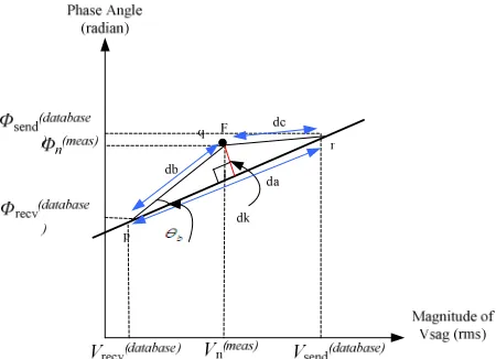
Voltage sag magnitude and phase angle are assumed as a linear function of a fault distance in ranking process. This assumption can be done for a short distance cables. To rank the possible faulted section among these selected sections, the rank algorithm will calculates the shortest distance between the measured sending and receiving voltage sags and the listed possible sections obtainable in database matching process. Formulation of dk is fundamentally formulated from trigonometric equation as follow;
(
)
2 2 2
2 cos
a b c b c b
d = d +d − ×d ×d ×
θ
(3)sin
k b c
d =d ×
θ
(4)Fig. 3. The Trigonometric Formulation in Estimating Shortest Distance, dk Due To Fault Occurrences (F)
C.Distance Estimation
As for the fault distance, impedance based method proposed by Adly A.Girgis [7] is used. This method utilized single measurement of voltage and current, which is formerly known as one-ended terminal at node prior to fault as displayed in Fig. 4. The distance is developed from single line to ground fault type.
0
select a
app
select a
V
V
Z
I
I
kI
=
=
+
(5)Equation (3.22) is expanded by substituting equation (3.21) into it and written as:
0 1
0
3 f
a
app
I R
Z DZ
I kI
= +
+
(6)
Equation (3.23) is expressed in the form of matrices with real and imaginary parts as follow:
2 1
1
2
2 1
1 2
f
app
app d s q s
d s q s
sm
sm
I I I I R
R I D
X I I I I R
X I
+
+ =
(7)
where,
(
)
2
1 2
d s q s
sm
I I
I I
L
I
+
=
(8)and
(
)
2
2 1
d s q s
sm
I I
I I
M
I
+
−
=
(9)Therefore final expression of distance is clarified as:
( )
( 1 1 ) a p p a p p
R M X L
D
R M X L
− =
− (10)
where,
0
I
is Zero sequence current at bus1
Z
is positive sequence impedances at line sectiona
V
is Phase voltage on phase a at busf
R is Fault resistance D is Distance to the fault (km)
[image:3.612.321.547.268.417.2]Major element of the proposed method is the updating magnitude of voltage and current on each node during faulty condition. The following Fig. 4 describes the updating voltage and current on node x prior to fault failure at node. The method starts from the measurement of V2 and I2, followed by obtaining the voltage drop via the branch admittance on bus x to find Vx. If fault occurred at other nodes after bus y under any circumstances, the process will restart and rise up continuously to an actual node determination before faulty node. The equation can be found in equation (11) and (12).
Fig. 4. The Determination of Updating Voltage and Current
The updating voltage
2
xabc abc d
V =V −V (11)
where,
Vxabc is Voltage at bus x
V2abc is Measuring voltage at main node Vd is Voltage drop in the line sections up to bus
The updating current
2
xabc abc ld
I =I −I (12)
where,
Ixabc is Current at bus x
I2abc is Measuring current at main node
Ild is Load current at bus y
select
app app app
select V
Z R jX
I
= = + (14)
1 2
I I jI
select = s + s (15)
comp d q
I
=
I
+
jI
(16)2 2 2
1 2
sm s s
I
=
I
+
I
(17)The equation of three phase balanced fault is clarified in equation (19) and (20).
(
)
(
)
app a b a b V V Z I I − = − (18)(
) (
)
I I I
comp a b
I I I I
a pf a b pf b
= ∆ − ∆
= − − −
(19)
where,
Zapp is Apparent impedance (Ω) Icomp is Compensating current (A)
Ispf, Ibpf is Pre-fault current at phase a, b and c (A) Ia, Ib is Fault current at phase a, b and c (A) Va is Fault voltage at phase a (V)
Vb is Fault voltage at phase b (V)
Z1 is Positive sequence impedance (Ω/km)
IV.RESULTS AND ANALYSIS A.Voltage Sag Profile
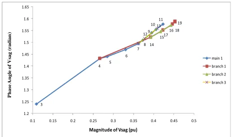
An identification of possible faulted section can be observed by characterizing the voltage sag profile on faulted nodes and lines. It is constructed based on fault occurrences created on all nodes and lines. Fig. 5 shows the magnitude and phase angle of the voltage sag, which lies in between the sending voltage magnitude and receiving voltage magnitude from the database of voltage sag magnitude and angle. When 3-phase balanced fault simulation is conducted on the six tested nodes and lines in the modelled network, it is observed that each node is distinguished through its individual pattern of voltage sag. Different pattern of voltage sag for main feeder 1, branch 1, branch 2 and branch 3 are illustrated from the graph plotted in Figure 4.5. The magnitude and phase angle of voltage sag increases gradually from the nearest nodes at main substation to the furthest nodes in the network configuration. The magnitude and angle of nodes 3 and 4 experiences shallow voltage sag on account of the adjacent location to the main nodes.
The potential faulted section in the network can be determined from the voltage sag pattern. For instance, nodes 3 and 4 are alone and non-overlapping with another section. Due to that, only one possible faulted section is selected.
[image:4.612.319.554.136.273.2]Other remaining nodes that have complicated voltage sag pattern that intersects with another section, there are possibilities of multiple faulty sections are selected. For instance, section 4-14 overlapped with sections 4-5, 5-6, 6-7, 7-8 along mainline 1. Hence, the tested sections of 4-5, 5-6, 6-7 and 6-7-8 will identify section 4-14 as one of their possible faulted section.
Fig. 5. Voltage Sag Magnitudes and Phase Angle for 3-Phase Balanced Fault
B.Result on Three Phase Fault
Three phase balanced fault is simulated in the modelled network. Table I indicates the simulation results on six differences tested nodes, whereby each node generates either one or multiple possible faulted sections depending on the voltage sag profile. Then, the ranking estimation formula is applied with priority being given to the lowest value of dk as the first rank. Only 1 faulted section at 8-9 is discovered at second attempt from six tested sections. This enables reducing time consumption concerning on physical inspection along the faulted feeder or sectionalized switching. Multiple possibilities of faulted section are generated at tested nodes of 4-5, 5-6, 6-7, 7-8 and 8-9 based on voltage sag pattern at Fig. 5.
In order to determine the performance and accuracy of the proposed algorithm, the error percentage of the actual fault distance and the calculated fault distance is evaluated follows.
%Error Dactual Dcalculated 100
Total Length of Main Feeder −
=
×
The fault distance and its percentage of error are display in column 5 and 7 respectively. It can be seen that for the fault section from node 4 to node 5, the actual distance is 0.14 km. However, using the proposed algorithm, the calculated distance of fault location is 0.1405 km. It is also shows the percentage error of the calculated fault distance over the actual distance for overall tested nodes are insignificant.
3 4 5 6 7 8 9 10 11 14 17 18 19 15 16 12 13 1.2 1.25 1.3 1.35 1.4 1.45 1.5 1.55 1.6 1.65
0.1 0.15 0.2 0.25 0.3 0.35 0.4 0.45 0.5
P h a se A n g le o f V sa g ( r a d ia n )
Magnitude of Vsag (pu)
TABLE I. TEST RESULT OF THREE PHASE FAULT ON NODES
3-4 3-4 1.25 0.0171 1.2542 1 √ 0.102
4-5 0.14 0.0006 0.1405 1 √
4-14 1.29 0.0029 1.2907 2
5-6 0.4 0.0027 0.3988 1 √
4-14 1.29 0.0121 1.2907 2
6-7 0.35 0.0009 0.351 1 √
4-14 1.29 0.0209 1.2907 2
7-8 0.2 0 0.1996 1 √
7-12 0.3 0.0001 0.2994 2
4-14 1.29 0.0107 1.2907 3
12-13 0.75 0.0002 0.7524 1
8-9 0.5 0.0003 0.4974 2 × 0.063 Tested
Nodes Fault Sections
Actual Distance
(km) dk
Calculated Distance
(km)
Ranking Attempt
Distance Error(%)
0.012
0.029
0.024
0.01 4-5
5-6
6-7
7-8
8-9
[image:5.612.317.551.95.303.2]C.Ranking Performance
Fig. 6 illustrates the observation of ranking performance; dk for both tested nodes and lines. Based on the ranking performed, most of the faulted nodes and lines appear in the first ranking attempt, which is also referred to as the first position, while the faulted sections 8-9 is found in the second ranking attempt. In the meantime, the tested sections such as 3-4 only lists one potential faulted section arising due to voltage sag independency.
Fig. 6. Numbers of Possible Fault Sections and Ranking Attempt for 3 Phase Balanced Fault
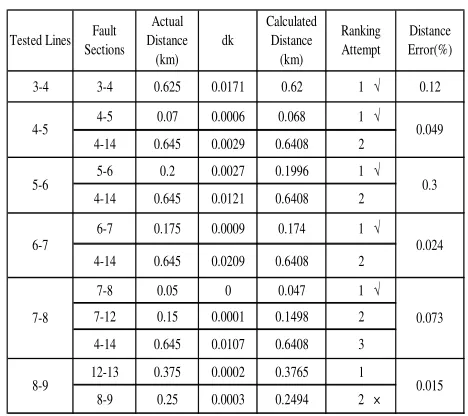
D.Faulted Lines
Table II shows the test outcome of three phase fault on six different lines. The fault is applied at the midpoint of each section in the network. Ranking results of tested lines is similar with tested nodes describes at Fig. 6. Although the calculated distance on the node line 3-4, 4-5, 5-6, 6-7, 7-8 and 8-9 is not equal with the actual fault location, the dissimilarity is approximated. The ability in locating fault
distance within the faulted section can improve the accuracy of fault location method.
TABLE II. TESTRESULTOFTHREEPHASEFAULTONLINES
3-4 3-4 0.625 0.0171 0.62 1 √ 0.12
4-5 0.07 0.0006 0.068 1 √
4-14 0.645 0.0029 0.6408 2
5-6 0.2 0.0027 0.1996 1 √
4-14 0.645 0.0121 0.6408 2
6-7 0.175 0.0009 0.174 1 √
4-14 0.645 0.0209 0.6408 2
7-8 0.05 0 0.047 1 √
7-12 0.15 0.0001 0.1498 2
4-14 0.645 0.0107 0.6408 3
12-13 0.375 0.0002 0.3765 1
8-9 0.25 0.0003 0.2494 2 × 0.015 0.049
5-6 0.3
6-7 0.024
7-8 0.073
Distance Error(%) Fault
Sections Actual Distance
(km) dk
Calculated Distance
(km)
Ranking Attempt Tested Lines
4-5
8-9
Fig.7 shows the distance error percentage for tested line of section 5-6 (blue solid line) and section 7-8 (red solid line) against actual distance. As shown in fig.7, distance error of shorted actual distance is approximately 0.25 % and 0.08 % for section 5-6 and section 7-8 respectively. The error percentage for section 5-6 gradually increases from 0.25 % - 0.52 % within the distance of 0.2 km – 0.4 km. For section 7-8, the error percentage gradually increases from 0.08 % - 0.32 % within the distance of 0.05 km - 0.2 km. The error percentage for both sections crosses at 0.28 % with actual distance of 0.18 km. Then, error percentage for section 7-8 gradually increases higher than section 5-6 with 0.13 % error percentage different at 0.2 km.
[image:5.612.68.288.402.541.2]Fig.7. Error Percentage of distance generated at section 5-6 and 7-8
V. CONCLUSION
This study has presented the combination of database approach and impedance based method to locate three phase balanced fault for non homogeneous distribution system. This algorithm only requires pre-fault and during fault in rms value of voltage and current at fundamental frequency before faulted point. Since this method only uses information from the measurement node, this algorithm can be considered as more simple and economical than the other fault location methods.
REFERENCES
[1] Hizman, H.; Crossley, P.A.; Gale, P.F.; Bryson, G.;, “Fault section identification and location on a distribution feeder using travelling waves,” Power Engineering Society Summer Meeting, 2002 IEEE, vol.3, no.,pp.1107-1112 vol.3, 25 July 2002.
[2] H. Mokhlis, A. H. A. Bakar, D. N. A.Talib, Hasmaini Mohamad, “The improvement of voltage sag pattern approach to locate fault a fault in distribution network”. International Review of Electrical Engineering (IREE), Vol.5 N.3, Part B, Page 1159-1164, June 2010.
[3] Karnik, N., Das, S., Kulkarni, S., & Santoso, S., "Effect of load current on fault location estimates of impedance-based methods," Paper presented at the IEEE Power and Energy Society General Meeting, 24-29 July 2011.
[4] Mora-Flòrez, J., Meléndez, J., & Carrillo-Caicedo, G. (2008)," Comparison of impedance based fault location methods for power distribution systems," Electric Power Systems Research, vol.78(4), pp.657-666.
[5] Short, T., Kim, J., & Melhorn, C.," Update on distribution system fault location technologies and effectiveness," Paper presented at the 20th International Conference and Exhibition on Electricity Distribution ,8-11 June 2009, Part 1. CIRED 2009.
[6] Mokhlis, H., Khalid, A. R., & Li, H. Y. ),"Voltage sags pattern recognition technique for fault section identification in distribution networks," Paper presented at the PowerTech, IEEE Bucharest.2009, June 28 -July 2 2009
[7] Girgis, A. A., Fallon, C. M., & Lubkeman, D. L. (1993)," A fault location technique for rural distribution feeder'". IEEE Transactions on Industry Applications, vol. 29, Issue.6, pp. 1170-1175
0 0.1 0.2 0.3 0.4 0.5 0.6
0 0.1 0.2 0.3 0.4 0.5
D
is
ta
n
c
e
E
r
r
o
r
(
%
)
Actual Distance (km)
Section 5-6