Mean Value Theorems for Harmonic Functions on the Cube in Rn

http://dx.doi.org/10.4236/apm.2015.511062

Mean-Value Theorems for Harmonic

Functions on the Cube in

_

n

Petar Petrov

Faculty of Mathematics and Informatics, Sofia University, Sofia, Bulgaria Email: [email protected]

Received 4 August 2015; accepted 13 September 2015; published 16 September 2015 Copyright © 2015 by author and Scientific Research Publishing Inc.

This work is licensed under the Creative Commons Attribution International License (CC BY).

http://creativecommons.org/licenses/by/4.0/

Abstract

Let

( )

{

n

}

n i

I r = x∈ x ≤r i, =1, 2,,n be a hypercube in n. We prove theorems concerning

mean-values of harmonic and polyharmonic functions on In

( )

r , which can be considered as

nat-ural analogues of the famous Gauss surface and volume mean-value formulas for harmonic func-tions on the ball in n

 and their extensions for polyharmonic functions. We also discuss an ap-plication of these formulas—the problem of best canonical one-sided L1_{-approximation by}

har-monic functions on In

( )

r .

Keywords

Harmonic Functions, Polyharmonic Functions, Hypercube, Quadrature Domain, Best One-Sided Approximation

1. Introduction

This note is devoted to formulas for calculation of integrals over the n-dimensional hypercube centered at 0

( )

{

}

: : n , 1, 2, , , 0,

n n i

I =I r = x∈ x ≤r i=  n r>

and its boundary Pn:=P rn

( )

:= ∂In

( )

r , based on integration over hyperplanar subsets of In and exact for

Let us remind that a real-valued function f is said to be harmonic ( polyharmonic of degree m≥2) in a given domain Ω ⊂n if f∈C2

( )

Ω

(

f ∈C2m

( )

Ω

)

and ∆ =f 0

(

m 0

)

f

∆ = on Ω, where ∆ is the Laplace operator and ∆m is its m-th iterate

(

)

2

1 2

1

: , : .

n

m m

i i f

f f f

x

−

=

∂

∆ = ∆ = ∆ ∆

∂

∑

For any set D⊂n, denote by H

( )

D

(

m

( )

, 2

)

D m≥

H the linear space of all functions that are har- monic (polyharmonic of degree m) in a domain containing D. The notation dλn will stand for the Lebesgue

measure in n.

2. Mean-Value Theorems

Let

( )

{

(

)

}

1 2 2 1

: n : n

n i i

B r = x∈ x =

∑

₌x ≤r and Sn

( )

r :=

{

x∈n x =r

}

be the ball and the hypersphere in n

 with center 0 and radius r. The following famous formulas are basic tools in harmonic function theory and state that for any function h which is harmonic on B r_n

( )

both the average over S_n

( )

r and the average over B r_n

( )

are equal to h 0

( )

.

The surface mean-value theorem.If h∈H

(

B rn

( )

)

, then

( )

(

)

( ) 1

( )

1

1

d ,

n n

S r n n

h h

S r σ

σ −

−

=

∫

0 (1)

where dσn−₁ is the

(

n−1

)

-dimensional surface measure on the hypersphere Sn

( )

r .

The volume mean-value theorem.If h∈H

(

B r_n

( )

)

, then

( )

(

)

( )

( )

1

d .

n n

B r n n

h h

B r λ

λ

∫

= 0 (2)

The balls are known to be the only sets in n satisfying the surface or the volume mean-value theorem. This means that if Ω ⊂n is a nonvoid domain with a finite Lebesgue measure and if there exists a point x₀∈ Ω such that

( )

( )

0

1

d n n

h h

λ

λ

Ω

=

Ω

∫

x for every function h which is harmonic and integrable on Ω, then Ω is an open ball centered at x₀ (see [4]). The mean-value properties can also be reformulated in terms of quadrature domains [5]. Recall that Ω ⊂n is said to be a quadrature domain for H

( )

Ω , if Ω is a connected open set and there is a Borel measure dµ with a compact support K_µ ⊂ Ω such that fd n _K fd

µ

λ

µ

Ω =

∫

∫

for every λ_n -integrable harmonic function f on Ω. Using the concept of quadrature domains, the volume mean-value property is equivalent to the statement that any open ball in n is a quadrature domain and the measure dµ is the Dirac measure supported at its center. On the other hand, no domains having “corners” are quadrature domains [6]. From this point of view, the open hypercube I_n is not a quadrature domain. Nevertheless, it is proved in Theorem 1 below that the closed hypercube I_n is a quadrature set in an extended sense, that is, we find explicitly a measure dµ with a compact support K_µ having the above property with Ω replaced by

n

I but the condition K_µ ⊂I_n is violated exactly at the “corners” (for the existence of quadrature sets see [7]). This property of I_n is of crucial importance for the best one-sided L1-approximation with respect to H

( )

I_n

(Section 3).

Let us denote by D_nij the

(

n−1

)

-dimensional hyperplanar segments of I_n defined by

( )

{

}

: : , , , 1 ,

ij ij

n n n k i j

D =D r = x∈I x ≤ x = x k≠i j ≤ < ≤i j n

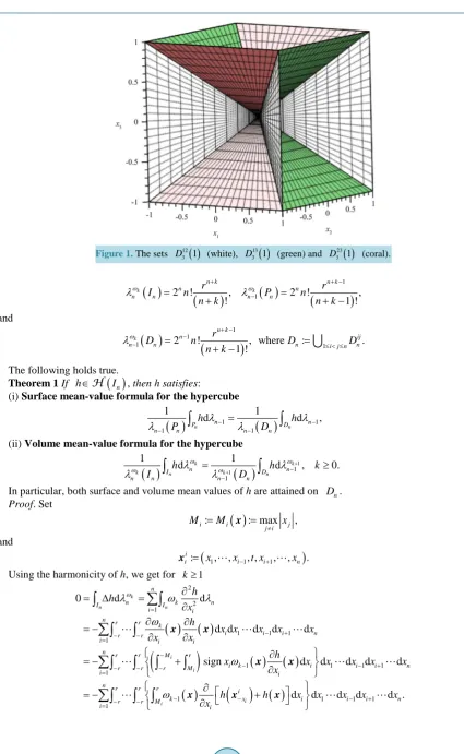
(seeFigure 1). Denote also

( )

(

max

{

1, 2 , ,

}

)

: , 0,

!

k n k

r x x x

k k

ω x = −  ≥

and d k : d

m k m ω

[image:3.595.89.515.66.758.2]

Figure 1. The sets 12

( )

3 1

D (white), 13

( )

3 1

D (green) and 23

( )

3 1

D _(coral).

( )

2 !

₍

₎

, 1

( )

2 !

₍

1

₎

,

! 1 !

k k

n k n k

n n

n n n n

r r

I n P n

n k n k

ω ω

λ = ₊+ λ− = _{+ −}+ −

and

( )

1

₍

1

₎

1 2 ! , where : 1 .

1 !

k

n k

n ij

n n n i j n n

r

D n D D

n k ω

λ − + −

− = _{+ −} =



≤ < ≤

The following holds true.

Theorem 1 If h∈H

( )

I_n , then h satisfies: (i) Surface mean-value formula for the hypercube

( )

1

( )

1

1 1

1 1

d d ,

n n n n

P D

n n n n

h h

P

λ

D

λ

λ

−

λ

−

− −

=

∫

∫

(3) (ii) Volume mean-value formula for the hypercube

( )

1

( )

11

1

1 1

d k d k , 0.

k In n k Dn n

n n n n

h h k

I D

ω ω

ω λ ω λ

λ λ + −+

−

= ≥

∫

∫

(4)

In particular, both surface and volume mean values of h are attained on D_n.

Proof. Set

( )

: : max ,

i i j

j i

M M x

≠

= x =

and

(

1 1 1

)

: , , , , , , .

i

t = x xi− t xi+ xn

x  

Using the harmonicity of h, we get for k≥1

( ) ( )

(

)

( ) ( )

( )

( )

( )

2

2 1

1 1 1

1

1 1 1 1

1

1 1

0 d d

d d d d d

sign d d d d d

d

k

n n

i i

i i

n

n k n

I I

i i

n _{r r}

k

i i i n

r r

i i i

n _{r r M r}

i k i i i n

r r r M

i i

n _{r r r}

i

k x i

r r M

i i

h h

x h

x x x x x

x x

h

x x x x x x

x

h h x

x ω

λ ω λ

ω

ω

ω

=

− +

− −

=

−

− − +

− − −

=

− −

− −

=

∂

= ∆ =

∂

∂ ∂

= −

∂ ∂

 ∂ 

= − _ + _

∂

 

 _{∂  }

= − _ + _

∂

∑

∫

∫

∑∫ ∫

∑∫ ∫ ∫

∫

∑∫ ∫ ∫

  

  



x x

x x

x x x dx₁ dx_i−1dx_i+1 d .x_n

 

Hence, we have

( ) ( )

( ) ( )

{

}

1 1 1

1

0 d d d d

i i

n _{r r}

i i i i

r r M M i i n

r r i

h − h + h − h + x x− x+ x

− −

=

 

= −

∑∫ ∫

 x + x −_ x + x _   (5) if k=1 and

( )

( )

( )

(

) (

) (

)

2 1 1 1

1

1 1 1 1

1

0 d d d d d

d d d d

i i

i i i

n _{r r r}

i

k x i i i n

r r M i

n _{r r}

i i i

k M M M i i n r r

i

h h x x x x x

h h x x x x

ω ω − − − + − − = − + − + − + − − =   = − _ + _   + _ + _

∑∫ ∫ ∫

∑∫ ∫

x x x

x x x

  

  

(6)

if k≥2.

Clearly, (5) is equivalent to (3) and from (6) it follows

2 1

1

0 d k d k 2 d k ,

n n n n n n

I h Ih Dh

ω ω ω

λ

λ

−

λ

−

−

= ∆

_∫

=

_∫

−

_∫

(7) which is equivalent to (4). □

Let M:=M

( )

x : max= ₁≤ ≤i n xi . Analogously to the proof of Theorem 1 (ii), Equation (7) is generalized to:

Corollary 1 If h∈H

( )

I_n and 2

[ ]

0,

C r

ϕ ∈ is such that

ϕ

( )

0 =0 and

ϕ

′

( )

0 =0, then

(

)

(

)

(

)

1

0 d d 2 d .

n n n n n n

I

ϕ

r M h

λ

I

ϕ

′′ r M h

λ

D

ϕ

′ r M h

λ

−

=

_∫

− ∆ =

_∫

− −

_∫

− (8)

The volume mean-value formula (2) was extended by P. Pizzetti to the following [2] [3] [8].

The Pizzetti formula.If g∈Hm

(

B rn

( )

)

, then

( )

(

)

( )

2 1 2 2 0

d π .

!

2 2 1

n k k m n n n k B r k g r g r k n k λ − = ∆ =

Γ + +

∑

∫

0

Here, we present a similar formula for polyharmonic functions on the hypercube based on integration over the set D_n.

Theorem 2 If g∈Hm

( )

I_n , m≥1, and ϕ ∈C2m

[ ]

0,r is such that

ϕ

( )k

( )

0 =0, k=0,1,, 2m−1, then the following identity holds true for any k≥0:

( )

₍

₎

1 ( )

₍

₎

2 2 1 1

1 0

d 2 d ,

n n

m

m s m s

n n

I D

s

r M g r M g

ϕ λ − ϕ + − − λ

− =

− =

∑

− ∆

∫

∫

(9)

where ( )

( )

d

( )

d j j j t t t ϕ

ϕ = .

Proof. Equation (9) is a direct consequence from (8):

(

)

( )

₍

₎

( )

₍

₎

( ) ( )

1 1 2 1

1 1

2 1 1 2 1 0

0 d

2 d d

2 d d .

n n n n n m n I m m n n D I m

s m s m

n n

D I

s

r M g

r M g r M g

g g

ϕ λ

ϕ λ ϕ λ

ϕ λ ϕ λ

− − − − + − − − = = − ∆ = − − ∆ + − ∆ = = − ∆ +

∫

∫

∫

∑∫

∫



3. A Relation to Best One-Sided

L

1

_{-Approximation by Harmonic Functions}

Theorem 1 suggests that for a certain positive cone in C I

( )

_n the set D_n is a characteristic set for the best one-sided L1-approximation with respect to H

( )

I_n as it is explained and illustrated by the examples presented below.

For a given f ∈C I

( )

_n , let us introduce the following subset of H

( )

I_n :

(

In,f

)

:

{

h

( )

In h f on .In

}

− = ∈ ≤

H H

A harmonic function _*f

(

,

)

n

(

)

* ₁

1 for every , , f

n

f −h ≤ f −h h∈H₋ I f

where

1: I_n d .n g =

∫

g

λ

Theorem 1 (ii) readily implies the following ([6] [9]).

Theorem 3 Let f ∈C I

( )

_n and _*f

(

,

)

n

h ∈H− I f . Assume further that the set Dn belongs to the zero set of the function f −h_*f . Then h_*f is a best one-sided L1-approximant from below to f with respect to H

( )

I_n .

Corollary 2 If 1

( )

n

f∈C I , any solution h of the problem

(

)

|Dn |Dn, |Dn |Dn, n, ,

h = f ∇h = ∇f h∈H− I f (10)

is a best one-sided L1-approximant from below to f with respect to H

( )

I_n .

Corollary 3 If

( )

( )

(

2 2

)

2

1i j n i j

f x =g x

∏

_{≤ < ≤} x −x , where g∈C I

( )

_n and g≥0 on I_n, then _*f

( )

0

h x ≡ is a best one-sided L1-approximant from below to f with respect to H

( )

I_n .

Example 1 Let n=2, r=1 and f₁

(

x x₁, ₂

)

=x x₁2 ₂2. By Corollary 2, the solution

(

)

1 4 2 2 4

* 1 2 1 1 2 2

3

, 4 4

2

f

h x x = −x + x x −x of the interpolation problem (10) with f = f₁ is a best one-sided L1- appro-ximant from below to f1 with respect to H

( )

I2 and 1 *1 ₁ 8 45

f

f −h = . Since the function f₁ belongs to the positive cone of the partial differential operator

4 4

2,2 2 2 1 2

:

x x

∂ =

∂ ∂

 (that is, 4 2,2 1f >0

 ), one can compare the best harmonic one-sided L1-approximation to f1 with the corresponding approximation from the linear sub-

space of C I

( )

2 :

( )

( ) (

)

1

( )

( )

2,2

2 2 1 2 0 1 2 1 2 1 0

: , j j j j .

j

I b C I b x x a x x a x x

=

 

 

= ∈ = _ + _



∑



B

The possibility for explicit constructions of best one-sided L1-approximants from 2,2

( )

2 I

B , is studied in [10]. The functions 1

1 * f f −b and

1 * 1 f

f −b , where 1 *

f b and

1 * f

b are the unique best one-sided L1-approximants to f1

with respect to 2,2

( )

2 I

B from below and above, respectively, play the role of basic error functions of the cano- nical one-sided L1-approximation by elements of 2,2

( )

2 I

B . For instance, 1 *

f

b can be constructed as the unique interpolant to f1 on the boundary ◊ =:

{

(

x x1, 2

)

∈I2 x1 + x2 =1

}

of the inscribed square and

1 1 *

1 14 45 f

f −b = (Figure 2).

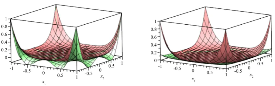
Example 2 Let n=2, r=1 and

(

)

8 4 4 8

2 1, 2 1 14 1 2 2

f x x =x + x x +x . The solution

(

)

(

)

2 8 8 6 2 2 6 4 4 * 1, 2 1 2 28 1 2 1 2 70 1 2

f

h x x =x +x − x x +x x + x x of (10) with f = f₂ is a best one-sided L1-approximant from below to f₂ with respect to H

( )

I2 and 2 *2 8 75

f

f −h = . It can also be verified that 2

2 * 121 900 f

f −b =

[image:5.595.107.527.549.683.2]

(seeFigure 3).

Figure 2. The graphs of the function f x x1

(

1, 2

)

=x x12 22 (coral) and its best one-sided L 1

-approximants from below,

1

*

f

h with respect to H I

( )

₂ (left) and 1

*

f

b with respect to 2,2

( )

2

I

[image:6.595.88.541.80.223.2]

Figure 3. The graphs of the function

(

)

8 4 4 8 2 1, 2 1 141 2 2

f x x =x + x x +x (coral) and its best one-sided L1-approximants from below, 2

*

f

h with respect to H

( )

I2 (left) and

2

*

f

b with respect to 2,2

( )

2

I

B (right).

Remark 1 Let ϕ ∈C2

[ ]

0,r is such that

ϕ

( )

0 =0,

ϕ

′

( )

0 =0, and ϕ′ ≥0, ϕ′′ ≥0 on

[ ]

0,r . It follows from (8) that Theorem 3 also holds for the best weighted L1-approximation from below with respect to H

( )

I_n

with weight

ϕ

′′ −

(

r M

)

. The smoothness requirements were used for brevity and wherever possible they can be weakened in a natural way.

References

[1] Helms, L.-L. (2009) Potential Theory. Springer-Verlag, London. http://dx.doi.org/10.1007/978-1-84882-319-8

[2] Pizzetti, P. (1909) Sulla media dei valori che una funzione dei punti dello spazio assume sulla superficie della sfera.

Rendiconti Linzei—Matematica e Applicazioni, 18, 182-185.

[3] Courant, R. and Hilbert, D. (1989) Methods of Mathematical Physics Vol. II. Partial Differential Equations Reprint of the 1962 Original. John Wiley & Sons Inc., New York.

[4] Goldstein, M., Haussmann, W. and Rogge, L. (1988) On the Mean Value Property of Harmonic Functions and Best Harmonic L1-Approximation. Transactions of the American Mathematical Society, 305, 505-515.

[5] Sakai, M. (1982) Quadrature Domains. Lecture Notes in Mathematics, Springer, Berlin.

[6] Gustafsson, B., Sakai, M. and Shapiro, H.S. (1977) On Domains in Which Harmonic Functions Satisfy Generalized Mean Value Properties. Potential Analysis, 71, 467-484.

[7] Gustafsson, B. (1998) On Mother Bodies of Convex Polyhedra. SIAM Journal on Mathematical Analysis, 29, 1106- 1117. http://dx.doi.org/10.1137/S0036141097317918

[8] Bojanov, B. (2001) An Extension of the Pizzetti Formula for Polyharmonic Functions.Acta Mathematica Hungarica, 91, 99-113. http://dx.doi.org/10.1023/A:1010687011674

[9] Armitage, D.H. and Gardiner, S.J. (1999) Best One-Sided L1-Approximation by Harmonic and Subharmonic Functions. In: Haußmann, W., Jetter, K. and Reimer, M., Eds., Advances in Multivariate Approximation, Mathematical Research (Volume 107), Wiley-VCH, Berlin, 43-56.