Analysis and Classification of EEG Signals based on a
New Quantum Inspired Wavelet Neural Network Model
Saleem M. R. Taha,
Ph.D. Department of Electrical Engineering, College of Engineering, University of Baghdad,Jadiryah, Baghdad, Iraq
Zahraa K. Taha,
M.Sc. Department of Electrical Engineering, College of Engineering, University of Baghdad,Jadiryah, Baghdad, Iraq
ABSTRACT
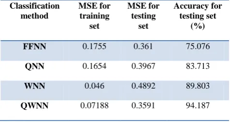
In this paper, electroencephalographic (EEG) signals are analyzed and classified based on a new multilevel transfer function quantum wavelet neural network (QWNN) model. The independent component analysis (ICA) is used as processing after normalization of these signals. Some features are extracted from the data using the clustering technique (CT). The classification result of the new model is compared with that of wavelet neural network (WNN), quantum neural network (QNN), and feed forward neural network (FFNN). The new QWNN model is found to achieve average classification accuracy of 94.187%, but classification accuracies using WNN, QNN and FFNN are 89.803%, 83.713% and 75.076%, respectively
General Terms
Pattern Recognition, Theory, Algorithms
Keywords
EEG Signals, Neural Networks, Quantum Computing, Wavelet Transforms, Wavelet Neural Networks
1.
INTRODUCTION
The electroencephalographic (EEG) examination is a standard procedure in the study of all forms of cerebral disease. Its use in the study of patients with seizures and those suspected of having seizures becomes essential [1].
The brain is an electrochemical organ. Its electrical activity (EEG) is easily recorded, amplified, and displayed [2]. The amplitude and frequency of EEG signals vary with human state (asleep or awake), age, health, etc. EEG represents the recording of spontaneous electrical activity of the brain. EEG signals are recorded in a short time, normally for 20-40 minutes. The electrodes are placed at various positions on the scalp to get the required recordings. It is believed that the EEG signals represent the status of the whole body, as well as the electrical signals of the brain [3], [4].
The EEG consists of a set of multichannel signals. The pattern of changes in signals indicates brain activities. In addition the EEG also reflects activation of the head musculature, eye movements, interference from nearby electrical devices, and changing conductivity in the electrodes due to the movements of the subject or physiochemical reactions at the electrode sites. All of these activities are referred to as background activities [5].
The amplitude of EEG signals is very low, varying between 5 and 100 mV. There are five categories of these signals: delta, theta, alpha, beta, and gamma. Each of which is associated with a certain activity of the brain.
EEG signals possess a combination of slow variations over long periods, with sharp, transient variations over short
periods. Hence, it seems that wavelet neural networks (WNNs) are the more suitable choice than other mainstream neural networks for EEG analysis. The aim of the paper is to develop a new quantum wavelet neural network (QWNN) model for the analysis and classification of EEG signals.
2.
QUANTUM NEURAL NETWORKS
QNN has an inherently fuzzy architecture which can encode the sample information into discrete levels of certainty/uncertainty. The goal is accomplished by using quantum neurons in the hidden layer of the network. The transfer function of the quantum neuron has the ability to form graded partitions in feature space. One possibility of obtaining this kind of transfer function is to take the superposition of ns sigmoidal functions, each shifted by quantum interval 𝜃𝑠 (s=1, 2, …, ns), where ns is called the total number of quantum levels [6].
Consider QNN with ni inputs, no output nodes and one layer of nh hidden nodes. Let 𝑣𝑙𝑗= [𝑣1𝑗, 𝑣2𝑗, … , 𝑣𝑛𝑖𝑗]
𝑇 be the
weight vector connection of the jth hidden node to the inputs and 𝑤𝑗𝑖= [𝑤1𝑖, 𝑤2𝑖, … , 𝑤𝑛𝑖]𝑇 be the weight vector connection of the ith output node to hidden nodes. Let the activation function of the hidden nodes be the sigmoid function𝑔𝑜: R → [0,1]. Then the input to the 𝑗𝑡 hidden node
from 𝑘𝑡 feature vector 𝑥𝑘 is ĥjk= 𝑛𝑙=1𝑖 𝑣𝑙𝑗𝑥𝑙𝑘. Suppose a
multi-level hidden node has 𝑛𝑠 discrete quantum levels. Then
its activation function can be written as a superposition of 𝑛𝑠
sigmoid functions, each shifted by 𝜃𝑠 [7].
𝑔 𝑥 =𝑛1
𝑠 𝑔𝑜 (𝛽 (𝑥 −
𝑛𝑠
𝑠=1 𝜃𝑠)) (1)
where 𝑔𝑜 𝑥 = 1 (1 + 𝑒−𝑥) is a sigmoid function, 𝛽 is a
slope factor of hidden function, and 𝜃𝑠 defined the jump-positions in activation function. Therefore, the response of the
𝑗𝑡 multi-level hidden unit to the 𝑘𝑡 feature vector 𝑥𝑘can be
written as [6] Ĥ𝑗𝑘=𝑛1
𝑠 𝑗
𝑘 𝑛𝑠
𝑠=1 = 1
𝑛𝑠 𝑔𝑜 (𝛽 (ĥj
k− 𝑛𝑠
𝑠=1 𝜃𝑗𝑠)) (2)
The response of the 𝑖𝑡 output nodes to the 𝑘𝑡 feature vector can be written as 𝑧𝑖𝑘 = 𝑓 ŷ𝑖𝑘 , where ŷ𝑘𝑖 = 𝑛𝑗 =1 𝑤𝑗𝑖Ĥ𝑗𝑘 and
𝑓 𝑥 = 𝑔𝑜 (𝛽𝑜 𝑥). 𝛽𝑜 is the slope factor of output function.
3.
THE LEARNING ALGORITHM OF
QNN
3.1
Updating the Weights in QNN
First should train the weights which involve presenting all the training set to the network and a forward pass and back propagation like a normal neural network. Let 𝑑𝑖𝑘= [𝑑1𝑘𝑑2𝑘𝑑𝑘3… 𝑑𝑛𝑘𝑜]𝑇 be the desired output vector for the 𝑘𝑡 input feature vector 𝑥𝑘= [𝑥1𝑘, 𝑥2𝑘, … , 𝑥𝑛𝑖
𝑘]. Let 𝑧
𝑖𝑘=
[𝑧1𝑘𝑧2𝑘𝑧3𝑘… 𝑧𝑛𝑘𝑜]𝑇 be the actual output. A gradient-descent-based algorithm for learning the synaptic weights of the QNN can be derived by minimizing the quadratic error function sequentially for each 𝑘 [8] ,[9].
𝐸𝑘=1
2 (𝑑𝑖 𝑘 𝑛𝑜
𝑖=1 − 𝑧𝑖𝑘)2 with 𝑘 = 1,2, … , 𝑚 (3)
Where 𝑧𝑖𝑘 is the actual output of the training pattern 𝑘 and
output 𝑖. 𝑑𝑖𝑘 is desired output of the training pattern 𝑘 and
output 𝑖. 𝑚 is the total number of the training pattern. E are mean square error functions.
Example-by-Example or on-line learning (in which the weights are adjusted after every training pattern) is used to update the weights.
The parameters 𝑣𝑙𝑗, 𝑤𝑗𝑖 are updated by minimizing objective
function 𝐸𝑘 [6]
∂E𝑘
𝜕𝑤𝑗𝑖 = 𝛽𝑜𝑒𝑖
𝑘𝑧
𝑖𝑘 1 − 𝑧𝑖𝑘 Ĥ𝑗𝑘 (4)
∂E𝑘
𝜕𝑣𝑙𝑗 = 𝛽𝛽𝑜 𝑒𝑖 𝑘𝑧
𝑖𝑘 1 − 𝑧𝑖𝑘 𝑛𝑜
𝑖=1 𝑤𝑗𝑖𝑛1
𝑠 𝑗
𝑠,𝑘 𝑛𝑠
𝑠=1 1 − 𝑗𝑠,𝑘 𝑥𝑙𝑘
(5)
Where 𝑒𝑖𝑘=𝑧𝑖𝑘− 𝑑𝑖𝑘.
At any epoch 𝑟, adjustment of parameters 𝑣𝑙𝑗, 𝑤𝑗𝑖 are
performed according to
w𝑗𝑖 𝑟 + 1 = w𝑗𝑖(𝑟) − 𝛼∂E
𝑘
∂w𝑗𝑖 (6)
v𝑙𝑗 𝑟 + 1 = v𝑙𝑗(𝑟) − 𝛼∂E
𝑘
∂v𝑙𝑗 (7) Where 𝛼 is the learning rate, 0 < 𝛼 < 1.
3.2
Updating the Quantum Intervals
The QNN must be first trained to recognize the occurrence of transitions between classes. The synaptic weights of the QNN must be updated to enable the network to learn the class boundaries on the feature space [9]. After that training the quantum intervals 𝜃𝑗𝑠, before the jump-positions are updated,
the training set is presented to the network. Once again to calculate <Ĥ𝑗𝑐𝑖> (it's the sum of outputs of hidden neurons for
all the inputs that belong to class 𝑐𝑖 divided by the number of
samples in that class). This is seem as a kind of forward pass, then 𝜃𝑗𝑠 is updated.
The idea of amendments to quantum intervals is to realize the minimal output variety of hidden layer neuron based on the same category of sample data, essentially, it’s also based on the negative gradient algorithm, and the samples at the fuzzy boundary which do not belong to the same category can be mapped to different class by this algorithm. The variance of the output of the 𝑗𝑡 hidden nodes for 𝑖𝑡 class is [10] 𝜎𝑗 ,𝑖2 = 𝑥𝑘𝜖𝑐𝑖(< Ĥ𝑗𝑐𝑖>− Ĥ𝑗𝑘)2 (8)
Where < Ĥ𝑗𝑐𝑖> = 1
𝐶𝑖 Ĥ𝑗
𝑘 𝑥𝑘𝜖𝑐𝑖
The adjustment of quantum intervals 𝜃𝑗𝑠 will be realized by
minimizing objective function G. 𝐺 =12 𝑛𝑗 =1 𝑛𝑖=1𝑜 𝜎𝑗 ,𝑖2 =
1
2 (< Ĥ𝑗
𝑐𝑖 >
𝑥𝑘𝜖𝑐𝑖 − Ĥ𝑗𝑘)2
𝑛𝑜
𝑖=1 𝑛
𝑗 =1
(9) The update equation for 𝜃𝑗𝑠 can be obtained by setting the change in 𝜃𝑗𝑠, say ∆𝜃𝑗𝑠 proportional to the gradient of G with
respect to 𝜃𝑗𝑠 as
∆𝜃𝑗𝑠= −𝛼𝜃𝜕𝜃𝜕𝐺
𝑗
𝑠 = (< Ĥ𝑗
𝑐𝑖>
𝑥𝑘𝜖𝑐𝑖 − Ĥ𝑗𝑘) [
𝜕<Ĥ𝑗𝑐𝑖> 𝜕𝜃𝑗𝑠 −
𝑛𝑜
𝑖=1 Ĥ𝑗𝑘
𝜕𝜃𝑗𝑠] (10)
Where 𝛼𝜃 is the learning rate, 0 < 𝛼𝜃< 1. The definition of
Equation (8) gives
𝜕<Ĥ𝑗𝑐𝑖> 𝜕𝜃𝑗𝑠 =
1 𝐶𝑖
𝜕Ĥ𝑗𝑘
𝜕𝜃𝑗𝑠
𝑥𝑘𝜖𝑐𝑖 (11)
𝜕Ĥ𝑗𝑘
𝜕𝜃𝑗𝑠=
−𝛽
𝑛𝑠 𝑗
𝑠,𝑘 1 − 𝑗𝑠,𝑘 = 𝑛𝑠
𝑠=1
−𝛽
𝑛𝑠 𝑣𝑗
𝑠,𝑘 𝑛𝑠
𝑠=1 (12)
Where 𝑣𝑗𝑠,𝑘= 𝑗𝑠,𝑘 1 − 𝑗𝑠,𝑘 , < 𝑣𝑗
𝑠,𝑐𝑖 > = 1
𝐶𝑖 𝑣𝑗
𝑠,𝑘 𝑥𝑘𝜖𝑐𝑖
Substituting Equations (11) and (12) into Equation (10) gives the update equation as:
∆𝜃𝑗𝑠= 𝛼𝜃𝛽𝑛
𝑠 (< Ĥ𝑗
𝑐𝑖 >
𝑥𝑘𝜖𝑐𝑖 − Ĥ𝑗𝑘)
𝑛𝑜
𝑖=1 (< 𝑣𝑗𝑠,𝑐𝑖 > −𝑣𝑗𝑠,𝑘)
(13)
The network is trained in a sequence of adaptation cycles. Each adaptation cycle involves the adaptation of all the internal parameters of the network, that is, the synaptic weights and the locations 𝜃𝑗𝑠 of the shifted and superimposed
sigmoid functions of the hidden units. Since the criterion employed for updating the parameters 𝜃𝑗𝑠 is based on all the
input vectors from the training set, 𝜃𝑗𝑠 are updated after the
presentation of all the inputs to the network and the corresponding adaptation of the synaptic weights [6].
4.
QUANTUM WAVELET NEURAL
NETWORK
The traditional neural networks have many disadvantages of slow speed, low accuracy convergence and shortcomings of generalization ability for pattern recognition. The concept of Quantum Neural Network (QNN) is developing in the 1990s; it can overcome the shortcomings and inadequacies of traditional neural network model by introducing quantum mechanics. QNN based on multilayer activation function is a three-layer network structure (input layer, hidden layer and output layer), where the input layer and output layer are the traditional feed forward neural networks while the quantum of hidden layer neurons borrowed the idea of superposition of quantum states in quantum theory. These QNNs are of very high theoretical value and application potential due to that they combine the respective advantage of neural computation and quantum computation.
comparison to assign it to all related categories if characteristic vector of sample is edge overlap which locates two types of modes. This make network have the feature of fuzziness and assign indeterminate data to all related categories.
5.
MODEL FOR QUANTUM WAVELET
NEURAL NETWORK
Quantum wavelet neural network (QWNN) is a new field which combines the quantum neural network (QNN) with wavelet theory. It is meaningful for QNN and classical neural network since will overcome some intractable problems and improve the network performance essentially. The incentive function of the hidden layer of QWNN uses superposition of nonlinear wavelet; here we selected Mexican hat functions. Such a hidden layer nodes can express more states [8]. The multilevel transfer function has several different quantum intervals, the different classes of data are mapped onto corresponding state; accordingly the classification has greater degree of freedom. Mexican hat wavelet has been chosen to serve as an adaptation basis function to network’s hidden layer for this QWNN, due to that data used correlates to the shape of the Mexican hat. As well the Mexican hat wavelets are continuous and differentiable wavelets respect to its dilation and translation parameters, the expression is as following:
𝜑 𝑡 = 1.373 ∗ (1 + 2𝜋𝑡2)𝑒−𝜋𝑡2
(14) As shown in Figure 1, the structure of QWNN includes three
layers. The input layer includes ni nodes, the hidden layer includes nh multilevel nodes and the output layer includes no nodes. Let the synaptic weight connection of the jth hidden nodes to the 𝑙𝑡 input be 𝑤𝑙𝑗. synaptic weight connection of
the ith output nodes to the jth hidden nodes be 𝑣𝑗𝑖. Let
𝑥𝑘= [𝑥
1𝑘, 𝑥2𝑘, 𝑥3𝑘, … , 𝑥𝑛𝑖𝑘]𝑇∀𝑘 = 1, … , 𝑚, where m is the number of the feature vectors of data set 𝑋. Suppose a multilevel hidden node has ns discrete quantum levels. Then
its activation function can be written as a superposition of ns
activation functions, each shifted by 𝜃𝑠,
𝑥 =𝑛1
𝑠 𝑜(𝛽 𝑥 − 𝜃
𝑠 ) 𝑛𝑠
𝑠=1 (15)
Where 𝑜(. ) is activation function, 𝛽 is slope factor, {𝜃𝑠} is
defined as the jump positions in the activation function. The step widths of the multilevel activation function, called the quantum intervals, are determined by jump positions {𝜃𝑠} .
Then the input to the jth hidden node from kth feature vector is ĥjk= 𝑛𝑙=1𝑖 𝑤𝑙𝑗𝑥𝑙𝑘. Therefore response of the jth multilevel
hidden node to the kth feature vector 𝑥𝑘 can be written as
𝐵𝑗 =𝑛1
𝑠 [𝛽 ĥj
k− 𝜃 𝑗𝑠 ] 𝑛𝑠
𝑠=1 𝑠 = 1,2, … , 𝑛𝑠 and
j=1,2,…,𝑛 (16)
Where h (•) = (𝑥𝑙−𝜏𝑗
𝜆𝑗 ) is the incentive function of hidden nodes, 𝜆𝑗 is dilation factor and 𝜏𝑗 is translation factor.
The output vector of output layer is
𝐶𝑖𝑘= 𝑛𝑗 =1 𝑣𝑗𝑖𝐵𝑗 , i=1,2,…,𝑛𝑜 (17)
The general model of the QWNN is
𝐶𝑖𝑘= 𝑛𝑗 =1 𝑣𝑗𝑖( 1
𝑛𝑠 (
(𝛽 ( 𝑛 𝑖𝑙=1𝑤𝑙𝑗𝑥𝑙)−𝜃𝑗𝑠 )−𝜏𝑗
𝜆𝑗
𝑛𝑠
𝑠=1 )) (18)
Where k is sample number.
The linear partition generated by an additional hidden node has all the degree of freedom to align itself along any direction on the feature space. On the other hand, the activation function within multilevel hidden nodes transfer function can only “spread-out” or “collapse-in” parallel to each other [10]. Another advantage could be reduction of the number of nodes in the hidden layer which could lead to a smaller number of weights [11].
6.
GRADIENT DESCENT BASED
LEARNING ALGORITHM FOR
QUANTUM WAVELET NEURAL
NETWORK
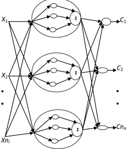
[image:3.595.317.527.332.578.2]The gradient descent based learning algorithm is easily computed, better for large data sets. Convergence of this algorithm depends on the learning rate α. If it is too large (such as constant) oscillation may occur. If it is too small, may not move far enough to reach a local minimum [12]. This can be done in two ways: example-by-example (or on-line learning), in which the weights are adjusted after every training pattern; and batch (or off-line) learning, in which learning weight adjustment occurs after all of the training examples have been presented to the network once [13].
Fig 1: Quantum wavelet neural network structure.
The learning of QWNN parameters is considered in two steps. The synaptic weights need to be updated first in order to train the QWNN to consistently partition the feature space of the given data set. Simultaneously, the uncertainty present in the feature space must be learned through the adaptation of the parameters 𝜃𝑟𝑠 [10].
6.1
Updating the Weights in QWNN
Let 𝑌𝑖𝑘= [𝑌1𝑘𝑌2𝑘𝑌3𝑘… 𝑌𝑛𝑜
𝑘]𝑇 be the desired output vector for
the kth input feature vector 𝑥𝑘 . Let 𝐶𝑖𝑘= [𝐶1𝑘𝐶2𝑘𝐶3𝑘… 𝐶𝑛𝑜
𝑘]𝑇
be the actual output vector. A gradient descent based algorithm for learning the synaptic weights of the QWNN can be derived by minimizing the quadratic error function sequentially for each k.
Σ Σ
Σ
X
1X
2C
2●
●
● ●
●
●
C
1Xn
i𝐸𝑘=1 2 (𝑌𝑖
𝑘 𝑛𝑜
𝑖=1 − 𝐶𝑖𝑘)2 (19)
Where k = 1, 2, …, m. 𝐶𝑖𝑘 is the actual output of the training
pattern k and output i. 𝑌𝑖𝑘 is the desired output of the training
pattern k and output i. m is the total number of the training pattern. E are mean square error functions.
The weights are adjusted after each feature vector 𝑥𝑘 is given as the input to the QWNN so that 𝐸𝑘 is minimized, this method called example-by-example or on-line learning. The advantages of this method are [12]:
It requires less computation per step.
Randomization may help escape poor local minima. It allows working with a stream of data rather than a
static set.
The parameters 𝑤𝑙𝑗, 𝑣𝑗𝑖, 𝜆𝑗, 𝜏𝑗 are updated by minimizing objective function 𝐸𝑘
∂E𝑘
∂V𝑗𝑖=𝑒𝑖*𝐵𝑗 (20)
∂E𝑘
∂w𝑟𝑗=𝑒𝑖v𝑗𝑖
1 𝑛𝑠
∂h ∂𝑥𝑙′
𝑛𝑠
𝑠=1 𝛽𝑥𝑙 (21)
𝑥𝑗′= 𝛽( 𝑛𝑙=1𝑖 𝑤𝑙𝑗𝑥𝑙− 𝜃𝑗𝑠)
Where
𝑡𝑗′= 𝑥𝑗′−𝜏
𝑗
𝜆𝑗 , 𝑒𝑖=𝐶𝑖
𝑘− 𝑌 𝑖𝑘
𝜕
𝜕𝑤𝑖𝑟= 1.373 ∗ 4𝜋𝑡 𝑒
−𝜋𝑡2
− 2𝜋𝑡 ∗ 1.373(1 + 2𝜋𝑡2)𝑒−𝜋𝑡2
(22) At any epoch h, adjustment of parameters 𝑤𝑙𝑗, 𝑣𝑗𝑖, 𝜆𝑗, 𝜏𝑗 are
performed according to
v𝑗𝑖 + 1 = v𝑗𝑖() − 𝛼∂E
𝑘
∂V𝑗𝑖 (23)
w𝑙𝑗 + 1 = w𝑙𝑗 − 𝛼∂E
𝑘
∂w𝑙𝑗 (24) Where 𝛼 is the learning rate, 0 < 𝛼 < 1.
6.2
Updating the Quantum Intervals
The quantum intervals of quantum nodes in the hidden layer can be learned by minimizing the class-conditional variances at the output of hidden nodes [14]. On other hand quantum intervals can be learned by minimal output variety of hidden layer node based on the same data category of sample data [10]. The output of variance for class 𝑐𝑖 is
𝜎𝑗 ,𝑖2 = 𝑥𝑘𝜖𝑐𝑖(< 𝐵𝑗 ,𝑐𝑖 >− 𝐵𝑗 ,𝑘)
2 (25)
Where < 𝐵𝑗 ,𝑐𝑖> =|𝑐1
𝑖| 𝑥𝑘∈𝑐𝑖𝐵𝑗 ,𝑘
< 𝐵𝑗 ,𝑐𝑖> is the sum of outputs of hidden nodes for all the
inputs that belong to class 𝑐𝑖 divided by the number of
samples in that class.
The adjusting of quantum intervals 𝜃𝑗𝑠 will be realized by
minimizing objective function G.
G=12 𝑛𝑗 =1 𝑛𝑖=1𝑜 𝜎𝑗 ,𝑖2 =12 𝑥𝑘𝜖𝑐𝑖(< 𝐵𝑗 ,𝑐𝑖>− 𝐵𝑗 ,𝑘) 2 𝑛𝑜 𝑖=1 𝑛 𝑗 =1 (26)
The update equation for 𝜃𝑗𝑠 can be obtained by setting the
change in 𝜃𝑗𝑠, say ∆𝜃𝑗𝑠proportional to the gradient of G with
respect to 𝜃𝑗𝑠 as:
∆𝜃𝑗𝑠= −𝛼𝜃𝜕𝜃𝜕𝐺
𝑗
𝑠= 𝑥𝑘𝜖𝑐𝑖(< 𝐵𝑗 ,𝑐𝑖 >− 𝐵𝑗 ,𝑘)[
𝜕<𝐵𝑗 ,𝑐𝑖>
𝜕𝜃𝑗𝑠 −
𝑛𝑜
𝑖=1 𝐵𝑗 ,𝑘
𝜕𝜃𝑗𝑠] (27) Where 𝛼𝜃 is the learning rate of 𝜃𝑗𝑠 𝑎𝑛𝑑 0 < 𝛼𝜃 < 1. 𝜕<𝐵𝑗 ,𝑐𝑖>
𝜕𝜃𝑗𝑠 =
1 |𝐶𝑗|
𝜕 𝐵𝑗 ,𝑘
𝜕𝜃𝑗𝑠
𝑥𝑘𝜖𝑐𝑖 (28)
𝜕 𝐵𝑗 ,𝑘
𝜕𝜃𝑗𝑠=
1 𝑛𝑠
𝜕 𝜃𝑗𝑠 = −
1 𝑛𝑠
𝜕
𝜕𝑋𝑖′𝛽 (29) Where
𝜕
𝜕𝑋𝑖′=[1.373 4𝜋𝑡 𝑒𝑥𝑝−𝜋𝑡 ′ 2
− 2𝜋𝑡 ∗
1.373 1 + 2𝜋𝑡2 𝑒𝑥𝑝−𝜋𝑡′ 2
]−1𝜆 𝑗 Let DB𝑗 ,𝑘=𝜕 𝐵𝜕𝜃𝑗 ,𝑘
𝑗𝑠 = −
𝛽 𝑛𝑠
𝜕
𝜕𝑋𝑖′ , and < DB𝑗 ,𝑘 > =
𝜕 < 𝐵𝑗 ,𝑐𝑖 >
𝜕𝜃𝑗𝑠 = −
𝛽 𝑛𝑠
1 𝐶𝑗
𝜕 𝜕𝑋𝑖′ 𝑥𝑘𝜖𝑐𝑖
Substitution of Equations (28) and (29) into Equation (27) gives the update equation as:
∆𝜃𝑗𝑠= −𝛼𝜃𝑛𝛽
𝑠 𝑥𝑘𝜖𝑐𝑖(< 𝐵𝑗 ,𝑐𝑖>− 𝐵𝑗 ,𝑘)
𝑛𝑜
𝑖=1 ∗ (< DB𝑗 ,𝑘>
−DB𝑗 ,𝑘) (30)
Where 𝛼𝜃 ∈ 0,1 is the learning ratio of 𝜃𝑗𝑠.
𝜃𝑗𝑠 can be updated according to the above equations:
(𝜃𝑗𝑠)+1= (𝜃𝑗𝑠)− 𝛼𝜃𝜕𝜃𝜕𝐺
𝑗𝑠 (31) Algorithm: Training The QWNN
Initialize all the parameters according to the above equations.
Update the synaptic weights: For k=1,2,…,m
For j=1,2,…, 𝑛
ĥjk= 𝑛𝑙=1𝑖 𝑤𝑙𝑗𝑥𝑙𝑘
𝑗𝑘,𝑠= 𝛽 ĥjk− θjs 𝑠 = {1,2, … , 𝑛𝑠}
𝐻𝑗𝑘𝑠= 𝑗𝑘𝑠−𝑡𝑗
𝜆𝑗 𝐵𝑗𝑘 =
1
𝑛𝑠 [ 𝐻𝑗 𝑘𝑠 ] 𝑛𝑠
𝑠=1
For i=1,2,….,𝑛𝑜
𝐶𝑖𝑘= 𝑛𝑗 =1 𝑣𝑗𝑖𝐵𝑗
For i=1,2,…,𝑛𝑜
𝑑𝑣𝑖𝑘= 𝑌𝑖𝑘− 𝐶𝑖𝑘
For j=1,2,…, 𝑛 and i=1,2,….,𝑛𝑜
v𝑗𝑖 = v𝑗𝑖− 𝛼𝑑𝑣𝑖𝑘𝐵𝑗𝑘
For j=1,2,3,…,𝑛
𝑑𝑤𝑗𝑘 = 1 𝜆𝑗∗
1 𝑛𝑠
𝜕 𝜕𝑡 𝑛𝑠
𝑠=1 𝐻𝑗𝑘𝑠 ∗ 𝑛𝑖=1𝑜 𝑑𝑣𝑖𝑘∗ 𝑣𝑗𝑖
For j=1,2,3,…,𝑛 and 𝑙 = 1,2, … , 𝑛𝑖
w𝑗𝑖= w𝑗𝑖− 𝛼 𝛽 𝑑𝑤𝑖𝑘𝑥𝑙𝑘
Update the quantum intervals: For k=1,2,…,𝑚
For j=1,2,…,𝑛
ĥjk= 𝑛𝑙=1𝑖 𝑤𝑙𝑗𝑥𝑙𝑘
𝑗𝑘,𝑠= 𝛽(ĥjk− θjs)𝑠 = {1,2, … , 𝑛𝑠}
𝐻𝑗𝑘𝑠= 𝑗𝑘𝑠−𝑡
𝑗
𝜆𝑗
𝐵𝑗𝑘 =𝑛𝑠1 𝑛𝑠=1𝑠 [ 𝐻𝑗𝑘𝑠 ]
For j=1,2,…,𝑛
< 𝐵𝑗 ,𝑐𝑖> = 𝑐1
𝑖 𝐵𝑗
𝑘 𝑥𝑘∈𝑐𝑖
< 𝐷𝐵𝑗𝑘,𝑠> = 1
𝑐𝑖 𝐷𝐵𝑗
𝑘,𝑠 𝑥𝑘∈𝑐𝑖
For k=1,2,…,m
For q=1,2,…,𝑛 and For s=1,2,…,𝑛𝑠
𝜃𝑞𝑠= 𝜃𝑞𝑠+ 𝛼𝜃𝑛𝛽
𝑠 < 𝐵𝑗 ,𝑐𝑖> −𝐵𝑗 𝑘 (< 𝐷𝐵
𝑗𝑘,𝑠 𝑥𝑘∈𝑐𝑖
𝑛𝑜
𝑖=1
> − 𝐷𝐵𝑗𝑘,𝑠)
7.
DATA SELECTION
From the data available at [15], the whole database consists of five EEG data sets (denoted A – E), each containing 100 single channel EEG signals of 23.6 seconds from five separate classes. Sets A and B consist of signals taken from surface EEG recordings of five healthy volunteers with eye open and eye closed, respectively. Signals in sets C and D were recorded in seizure-free intervals from five epileptic patients from the hippocampal function formation of the opposite hemisphere of the brain and from within the epileptic zone, respectively. Set E contains the records of five epileptic patients during seizure activity. All EEG recordings were made with the same 128-channel amplifiers system, using an average common reference [14]. The recorded data are digitized at 173.61 samples per second using 12-bit resolution. Band-pass filter setting is 0.53-40 Hz (12 dB/oct). The amplitude of EEG recordings is given in micro volt.
8.
CLASSIFICATION OF EEG SIGNAL
The classification operation of EEG signals can be divided into three stages. Stage one is used to process raw EEG signals in such a way that they are ready to be used. Stage two is feature extraction by cluster technique (CT). The last stage is EEG signal classification by QWNN.
8.1
Normalization
Normalization is a process to simplify the data. Each feature should be normalized (rearrange the data to range between 0 and 1) before the processing.
8.2
Data Processing
Raw EEG data is generally a mixture of several things: brain activity, eye blinks, muscle activity, environmental noise, etc. After the data have been collected, the preprocessing step starts to remove all noise and artifacts from the signal, but preserving all the characteristics of the original signal. As well as cleaning the signal from the influence of the reference electrode, if one is used [16].
All the above can be performed using different methods and algorithms, but Independent Component Analysis (ICA) is the best method for processing EEG signals. ICA is adequate if the data are no Gaussian, nonlinear, and no stationary [17]. EEG signal has all these properties, therefore ICA is used. A simple definition of the ICA problem can be given by reducing the problem to two original signal sources, s1 and s2, and two recorded mixtures, x1 and x2. The mixtures of the two sources are given by:
𝑥1(𝑛) = 𝑎11𝑠1 𝑛 + 𝑎12𝑠2 𝑛 (32)
𝑥2(𝑛) = 𝑎13𝑠1 𝑛 + 𝑎14𝑠2 𝑛 (33)
Where 𝑎11, 𝑎12, 𝑎13, and 𝑎14 are parameters that depend on
the position and characteristics of the recording locations [18]. The problem is now defined as solving for the source signals s1 and s2 using only mixtures x1 and x2.
8.3
Feature Extraction
Feature extraction is the process of extracting useful information from the signal. Features are characteristics of a signal that are able to distinguish between normal and abnormal of EEG signals. The requirements for feature extraction are [19]:
reduce the size of the data by selecting appropriate features,
the selected features should be minimally redundant and the expected results should maximally depend on these features,
preserve all information from the signal that is needed for classification.
It is basically impossible to apply any classification method directly to EEG samples, because of the large amount and the high dimension of the examples to describe such a big variety of clinical situation. There are many methods (feature extraction) used for this purpose [20].
Cluster technique (CT) is used to characterize brain activities from recording, several features are computed from the segmented data. These features allow representing each segmented data as a point in input vector space. The CT method is proposed for feature extraction from the original EEG database. This approach is conducted in three steps, which determines different clusters, sub clusters and statistical features extracted from each sub cluster, respectively. The steps of CT approach are:
1) Step 1: Each EEG data is divided into n groups, which are called clusters with specific time interval. 2) Step 2: Each cluster is partitioned into m sub
clusters with a specific duration.
3) Step 3: Eight statistical features are extracted from each sub cluster data point. The statistical features are minimum, maximum, mean, median, first quartile range, third quartile range, inter-quartile range, and standard deviation of the EEG data.
9.
EXPERIMENTS ON EEG SIGNALS
The epileptic EEG data have five sets, set A to set E. Each set contains 100 channels of data. Every channel consists of 4096 data points with 23.6 seconds. Each channel data is normalized and then divided into 16 groups, where each group is called cluster. Each cluster consists of 256 data points of 1.475 seconds. Then every cluster is again partitioned into sub clusters and each sub cluster contains 64 observations of 0.3688 second. Eight statistical features are calculated from each sub cluster. These features are the input for each of four different techniques applied to classify EEG signals. These techniques are Feed Forward Neural Network (FFNN), Quantum Neural Network (QNN), Wavelet Neural Network (WNN), and finally the new model of Quantum Wavelet Neural Network (QWNN).
is called testing samples. The testing samples are the remainder 30% of data, from which the error and accuracy of testing data are usually calculated. The performance of a particular run of the program, or a particular reading by an expert is evaluated in terms of the accuracy of classification, where:
𝐴𝑐𝑐𝑢𝑟𝑎𝑐𝑦 =𝑇𝑜𝑡𝑎𝑙 𝑛𝑢𝑚𝑏𝑒𝑟 𝑜𝑓 𝑐𝑜𝑟𝑟𝑒𝑐𝑡 𝑐𝑙𝑎𝑠𝑠𝑖𝑓𝑖𝑐𝑎𝑡𝑖𝑜𝑛𝑠𝑇𝑜𝑡𝑎𝑙 𝑛𝑢𝑚𝑏𝑒𝑟 𝑜𝑓 𝑡𝑒𝑠𝑡𝑖𝑛𝑔 𝑠𝑎𝑚𝑝𝑙𝑒𝑠 ∗ 100%
(34)
10.
RESULTS OF QUANTUM
WAVELET NEURAL NETWORK
MODEL
In this work, the data has been divided into two parts: the learning part and the testing part. Each trial is composed of feature vectors. The selection of the patterns for training and testing was made randomly. Training was conducted until standard of error fell below 0.0001 or a maximum iteration limit of 200 was reached. The mean square error (MSE) denotes the error limit to stop QWNN training.
A three layer structure of QWNN is applied. It consists of 32 inputs, 2 outputs, and 64 hidden layer nodes. The slope factor of multilevel transfer function is chosen to be 1.25 by trial and error.
The number of levels in quantum hidden layer will be chosen as a compromise between increased efficiency or increased computation cost. We will choose ns=10. We can choose greater than this but that will increase computation cost. The data must be dividable by the number of your choice because feature space cannot be divided into two regions and a half. The experiment results demonstrate that our proposed QWNN classifier achieves excellent performance in terms of classification accuracy compared to FFNN, QNN, and WNN; that will be discussed fully in the next section. As shown in Table 1, the average accuracy of 94.187% is obtained over 200 iterations. The average of MSE is 0.07188 decreasing with the increase of the number of iterations which means that the network is convergence to a solution as iterations number increases.
11.
DISCUSSION
[image:6.595.308.547.105.314.2]An epileptic EEG data is used in this work to test the performance of the proposed QWNN model. All calculations are performed using MATLAB (version 7.0.019920.R14). Here, different pairs of two-class EEG signals from five data sets in epileptic EEG data are to be classified. 1600 vectors of 32 dimensions (the dimensions of the extracted features) are obtained from each data set. 2240 vectors are used for training and 960 vectors for testing.
Table 1. Performance of QWNN for different pairs of two-class EEG signal from the epileptic EEG data
Different pairs
MSE for training set
MSE for testing set
Accuracy for testing set (%)
Sets A and E
0.0448 0.3054 97.946
Sets B and E
0.0711 0.3572 95.535
Sets C and E
0.0629 0.2292 95.758
Sets A and D
0.1231 0.5907 84.062
Sets D and E
0.0575 0.3130 97.633
Average 0.07188 0.3591 94.187
The proposed QWNN model is the most efficient to classify EEG signals. It is important to note that the EEG data from sets A and E are more classifiable than the other cases, because there are large variations among the recorded EEG. Due to the nature of large differences, it is easier to classify set A and set E as demonstrated by 97.946% accuracy of classification. In this application, the pair of sets A and D produce lowest classification accuracy of 84.062%.
The result of the experiments shows that the proposed QWNN model has improved the classification accuracy compared to the FFNN, QNN, and WNN classifiers. Table 2 illustrates this fact.
FFNN produces the lowest classification accuracy of 75.076% among the reported methods, because it creates its internal representations from sample information provided by training data. Training from sample data means that if a training vector belongs to the ith class, the ith output unit is required to respond with 1 while the responses of all other output units are required to be 0. The disadvantage of FFNN as compared with other methods is that, it is incapable of allowing the sample information to be encoded into certain levels (graded) of certainty/uncertainty.
The classification of QNN based on multilayer activation function is of more freedom than traditional FFNN, because activation function of the hidden nodes has a number of different quantum intervals. By adjusting the quantum intervals, the different classes of data are mapped onto corresponding state; accordingly the classification has more freedom. This is clear from Table 2, where the average accuracy of QNN is 83.713% while it is 75.076% for FFNN. WNN is fast, simple, robust, and reliable. Its classification accuracy is better than QNN and FFNN. WNN overcomes the problem of the sigmoid activation functions of QNN by using wavelet as activation function. But WNN has not inherently fuzzy architecture; therefore it should not be capable of generalizing the sample information into various graded levels of certainty over the entire feature space.
thus making the network clearer, simpler, and greatly reduces the size of the network and improve the learning speed. The other advantages of QWNN are overcoming the problems of slow speed and low accuracy of convergence and the shortcomings of generalization ability for pattern recognition of the traditional neural network.
TABLE 2. Comparison of EEG classification results
Classification method
MSE for training
set
MSE for testing
set
Accuracy for testing set
(%)
FFNN 0.1755 0.361 75.076
QNN 0.1654 0.3967 83.713
WNN 0.046 0.4892 89.803
QWNN 0.07188 0.3591 94.187
Replacing sigmoid function in QNN with Mexican hat wavelet basis function in QWNN solves the problem of QNN that the shape of sigmoid function is not identical to the shape of EEG signal. Mexican hat wavelet is often used for time-frequency analysis of EEG signals, because it can capture EEG events well. Another key advantage of Mexican hat wavelet is that it will manage to detect the great changes in EEG signals. Therefore, Mexican hat mother wavelet is used as activation function to provide considerable flexibility in designing the QWNN. Experiments show that the average accuracy is 94.187% for QWNN, whereas it is 83.713% for QNN. Also, the advantage of QWNN over FFNN is that if the eigenvectors of samples are located in the overlap edges of two modes, the QWNN will distribute them to all the relevant categories in proportion. The responses of the hidden nodes to input segments from the training and testing sets indicate that the trained QWNN and QNN produce a more structured internal representation of input samples than that produced by the trained WNN and FFNN. This experimental result was justified by illustrating the ability of trained QWNN and QNN to implement a multilevel partition of the input space.
12.
CONCLUSION
This paper presents a new QWNN model with Mexican hat as incentive function applied for classification of EEG signals. It overcomes the problems of slow speed and low accuracy of convergence and the shortcomings of generalization ability for pattern recognition of the traditional neural network. The combination of QNN with wavelet makes the network clearer and greatly reduces the size of the network, as well as improving the learning speed. Since we can choose the suitable basis function for the data in QWNN, therefore QWNN is more flexible than the other methods. In addition, this paper presents a learning algorithm. The validity of the model and the study algorithm are proved by simulation. The results proved that QWNN combined the theory of quantum superposition with wavelet theory can improve the accuracy and accelerate the speed of convergence. QWNN can classify the pattern precisely, and provides a method for those two modes which have overlap edges with difficulty to classify.
13.
REFERENCES
[1] Ropper, A. H., and Brown, R. H. 2011 Adams and Victor’s Principles of Neurology.8th ed.
[2] Hauser, S. L., and Josephson, S. A. 2011 Harrison Neurology in Clinical Medicine, 2nd ed. San Francisco: University of California.
[3] Verma, A. K., and Mangaraj, A. K. 2010 Analysis and Classification of Electroencephalography Signals. M.Sc. thesis, Electrics and Communication Eng. Dept., National Institute of Technology, Rourkela.
[4] Adikarapatti, V. 2007 Optimal EEG Channels and Rhythm Selection for Task Classification. Madras University, India, April 2007.
[5] Bartosova, V., Vysata, O. and Prochazka, A. 2006 Graphical User Interface for EEG Signal Segmentation. Computing and Control Eng. Dept., Institute of Chemical Technology.
[6] Zhou, J., Gan, Q., Krzyzak, A., and Suen, C. Y. 1999. Recognition of handwriting numerals by quantum neural network with fuzzy features. International Journal on Document Analysis and Recognition, ©Springer-Verlag, no. 2, 30-36.
[7] Karayiannis, N. B., Mukherjee, A., Glover, J. R., Frost, Jr, J. D., Hrachovy, R. A., and Mizrahi, E. M. 2005. An evaluation of quantum neural networks in the detection of epileptic seizures in the neonatal electroencephalogram. Soft Comput., Springer-Verlag,(10 May 2005).
[8] Liu, K., Peng, L. and Yang, O. 2010. The algorithm and application of quantum wavelet neural networks. in 2010 Chinese Control and Decision Conference, pp. 2941-2945.
[9] Karayiannis, N. B. and Purushothaman, G. 1997 Quantum neural networks (QNN’s): inherently fuzzy feed forward neural networks. IEEE Trans. Neural Networks. vol. 8, no. 3, May 1997.
[10] Xianwen, R., Feng, Z., Lingfeng, Z. and Xianwen, M. 2010. Application of quantum neural network based on rough set in transformer fault diagnosis. In Proc. Asia-Pacific Power and Engineering Conference, 2010, pp. 1-4.
[11] Malinowski, A., Cholewo, T. J. and Zurada, J. M. 1995. Capabilities and limitations of feed forward neural networks with multilevel neurons. In Proc. of the IEEE International Symposium on Circuits and Systems, vol. 1, Seattle, Wash., USA, April 1995, pp. 131-134.
[12] (2005, September 6).More on regression gradient descent classification (COMP-652,Lecture2)[Online].Available: http://www.facweb.iitkgp.ernet.in/~sudeshna/courses/M L06/regression-mcgill.pdf,
[13] Samarasinghe, S. 2006 Neural Networks for Applied Sciences and Engineering From Fundamental to Complex Pattern Recognition. Mechanical Eng. Dept., Lumumba Univ.
[15] (2005, November). EEG time series (epileptic data).[Online].
Available:http://www.meb.Unibonn.de/epileptologie/scie nce/physikleegdata.html
[16] Horlings, R. 2008 Emotion Recognition Using Brain Activity. Faculty Electrical Engineering, Mathematics, and Computer Science, Man-machine Interaction Group, Delft University of Technology, March 2008.
[17] Principal component analysis (PCA) and independent component analysis (ICA). [Online]. Available:http://www.cis.hut.fi/projects/ica/fastica/
[18] Faul, S. D. 2007 Automated Neonatal Seizure Detection. M.Sc. thesis, Electrical and Electronic Eng. Dept., National University of Ireland, Cork, 1st August 2007.
[19] Feature extraction and selection methods. [Online].Available:http://www.isa.umh.es/asignaturas/cs cs/PR/3%20-%20Feature%20extraction.pdf