Application of Mixture Models for Analyzing Reliability Data: A Case Study

How to cite this paper: Ruhi, S. (2015) Application of Mixture Models for Analyzing Reliability Data: A Case Study. Open Access Library Journal, 2: e1815. http://dx.doi.org/10.4236/oalib.1101815

Application of Mixture Models for Analyzing

Reliability Data: A Case Study

Sabba Ruhi

Department of Mathematics, Pabna University of Science and Technology, Pabna, Bangladesh Email: [email protected]

Received 18 August 2015; accepted 3 September 2015; published 9 September 2015

Copyright © 2015 by author and OALib.

This work is licensed under the Creative Commons Attribution International License (CC BY).

http://creativecommons.org/licenses/by/4.0/

Abstract

Whenever purchasing durable goods, customers expect it to perform properly at least for a rea-sonable period of time. Over the last 30 years there has been a heightened interest in improving quality, productivity and reliability of manufactured products. As discussed by Murthy, Xie and Jiang, [1] analyzed “Aircraft windshield failure data” and fitted 2-fold Weibull mixture model for this data set. They estimated the model parameters from WPP plot. In this study, a set of competi-tive 2-fold mixture models (including Weibull, Exponential, Normal, Lognormal, Smallest extreme value distribution) are applied to find out the suitable statistical models. The data consist of both failure and censored lifetimes of the windshield. In the existing literature, there are many uses of mixture models for the complete data, but very limited literature available about it uses for the censored data case. Maximum likelihood estimation method is used to estimate the model para-meters and the Akaike Information Criterion (AIC), Anderson-Darling (AD) and Adjusted Ander-son Darling (AD*) test statistics are applied to select the suitable models among a set of competi-tive models. Various characteristics of the mixture models, such as the cumulacompeti-tive distribution function, reliability function, mean time to failure, B10 life, etc. are estimated to assess the relia-bility of the component.

Keywords

Case Study, Data Analysis, EM Algorithm, Mixture Model, Reliability

Subject Areas: Mathematical Statistic

1. Introduction

OALibJ | DOI:10.4236/oalib.1101815 2 September 2015 | Volume 2 | e1815 about the average life span of their products. Again for costly items, customers expect that the product will per-form properly for a minimum life span without any disturbance. If this happens, the producer or his agent should give free service to repair or replace the item. Improving reliability of product is an important part of improving product quality. In recent years many manufacturers have collected and analyzed field failure data to improve the quality and reliability of their products and to develop customer satisfaction.

In this article we have considered both the nonparametric and parametric estimation procedures. The Akaike Information Criterion (AIC), Anderson-Darling (AD), Adjusted Anderson Darling (AD*), Root Mean Square Error (RMSE) & Kolmogrov-Smirnov test statistics (KSts) are applied to select the best models for the data sets. This article deals with the analysis of product failure data to estimate a variety of quantities of interest used in investigating product reliability.

The article is organized as follows: Section 2 describes the product failure data sets which will be analyzed in this paper. Section 3 derives the lifetime models. Section 4 explains the parameter estimation procedures of the lifetime models of the components. Section 5 discusses the results obtained from the analysis. Finally, Section 6 concludes the article with additional implementation issues for further research.

2. Data Set

Field failure data is superior to laboratory test data, because, it contains valuable information on the performance of any goods in actual usage conditions. There are many sources of collecting product reliability data. Warranty claim data is used as an essential source of field failure data which can be collected economically and efficiently through repair service networks and therefore, different procedures have been developed for collecting and ana-lyzing warranty claim data refer to the literatures [2]-[7].

Aircraft Windshield Failure Data

Failures of the Aircraft Windshield involve damage or delamination of the nonstructural outer ply or failure of the heating system. These failures do not result in damage to the aircraft but do result in replacement of the windshield.

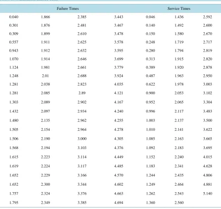
Data on failure and service times for a particular model windshield are given in Table 1 from “Murthy, Xie and Jiang [1]”, originally given in Blischke and Murthy [8]. The data consist of 153 observations. Among them 88 are classified as failed windshields, and the remaining 65 are censored time, means that had not failed at the time of observation. The unit for measurement is 1000 h.

3. Modeling

In the real world, problems arise in many different contexts. Always models play an important role in solving the problem. A variety class of statistical models have been developed and studied extensively in analyzing the product failure data [1] [4] [8]-[11]. The models that will be used to analyze the product failure data, given in Table 1, are discussed below.

Mixture Models

A general k-fold mixture model involves k subpopulations and is given by

( )

( )

1 1

, 0, 1

k k

i i i i

i i

G t p F t p p

= =

=

∑

>

∑

= (1)

where F ti

( )

is the CDF of the i-th sub-population and pi is the mixing probability of the i-th sub-population.

The density function is given by:

( )

( )

1 k

i i

i

g t p f t

=

=

∑

(2)

where f ti

( )

is the density function associated with Fi(t).

The hazard function h(t) is given by

( )

( )

_{( )}

( ) ( )

1

1

k

i i

i

g t

h t w t h t

G t =

= =

[image:3.595.89.537.93.515.2]

OALibJ | DOI:10.4236/oalib.1101815 3 September 2015 | Volume 2 | e1815

Table 1.Windshield failure data.

Failure Times Service Times

0.040 1.866 2.385 3.443 0.046 1.436 2.592

0.301 1.876 2.481 3.467 0.140 1.492 2.600

0.309 1.899 2.610 3.478 0.150 1.580 2.670

0.557 1.911 2.625 3.578 0.248 1.719 2.717

0.943 1.912 2.632 3.595 0.280 1.794 2.819

1.070 1.914 2.646 3.699 0.313 1.915 2.820

1.124 1.981 2.661 3.779 0.389 1.920 2.878

1.248 2.01 2.688 3.924 0.487 1.963 2.950

1.281 2.038 2.823 4.035 0.622 1.978 3.003

1.281 2.085 2.89 4.121 0.900 2.053 3.102

1.303 2.089 2.902 4.167 0.952 2.065 3.304

1.432 2.097 2.934 4.240 0.996 2.117 3.483

1.480 2.135 2.962 4.255 1.003 2.137 3.500

1.505 2.154 2.964 4.278 1.010 2.141 3.622

1.506 2.190 3.000 4.305 1.085 2.163 3.665

1.568 2.194 3.103 4.376 1.092 2.183 3.695

1.615 2.223 3.114 4.449 1.152 2.240 4.015

1.619 2.224 3.117 4.485 1.183 2.341 4.628

1.652 2.229 3.166 4.570 1.244 2.435 4.806

1.652 2.300 3.344 4.602 1.249 2.464 4.881

1.757 2.324 3.376 4.663 1.262 2.543 5.140

1.795 2.349 3.385 4.694 1.360 2.560

where hi(t) is the hazard function associated with subpopulation i, and

( )

( )

( )

1

( )

1

, 1

k

i i

i k i

i

i i

i

p R t

w t w t

p R t =

=

=

∑

=

∑

(4)

with

( )

1

( )

, 1

i i

R t = −F t ≤ ≤i k (5)

From (4), we see that the failure rate for the model is a weighted mean of the failure rate for the subpopula-tions with the weights varying with t.

Special Case: Two-Fold Mixture Model (k = 2) The CDF of the two-fold mixture model is given by

( )

1

( ) (

1

) ( )

2

G t = pF t + −p F t (6)

OALibJ | DOI:10.4236/oalib.1101815 4 September 2015 | Volume 2 | e1815

( )

1 exp t exp t exp t

G t p p

β

η θ θ

 _{ }  _{     }

= − −_{ } + _−_{ }− _−_{ }

   

       

  (7)

The probability density function g t

( )

is:

( )

t 1exp t

(

1 p

)

exp t

g t p

β β

β

η η η θ θ

−  _{ } _{  } _ _{−   }   = _   −  _+ − _{ }           (8)

Other two-fold mixture models can be derived by using different CDFs in (6) from different lifetime distribu-tions, similarly.

4. Parameter Estimation Procedures

In this article we have applied both the nonparametric (Kaplan-Meier estimate) and parametric (Weibull Proba-bility paper plot and maximum likelihood method) estimation procedures. The Akaike Information Criterion (AIC), Anderson-Darling (AD), adjusted Anderson Darling, Root Mean Square Error (RMSE) & Kolmogrov- Smirnov test statistics (KSts) are applied to select the best fitted models for the data sets.

4.1. Weibull Probability Paper Plot (WPP Plot)

In the early 1970s a special paper was developed for plotting the data under this transformation and was referred to as the Weibull probability paper (WPP) and the plot called the WPP plot. Weibull Probability Paper plot (WPP plot) is a special case of the probability paper plot. It is based on the Weibull transformations:

( )

{

}

( )

ln ln 1 and ln

y= − _ −F t _ x= t

A plot of y versus x is called the Weibull probability plot.

4.2. Maximum-Likelihood Estimation of Lifetime Model Parameters Random Censoring For censored data the likelihood function is given by

( )

( )

( )

1

1 i i n i i i

L λ f t δ R t −δ

=

 

=

∏

_{ }

where δiis the failure-censoring indicator for ti (taking on the value 1 for failed items and 0 for censored).

Tak-ing log on both sides we get,

( ) (

)

( )

{

}

1

ln ln 1 ln

n

i i i i

i

L δ f t δ R t

=

   

=

∑

_{ }+ − _{ } (9)

In the case of Weibull-Exponential mixture model putting the value of CDF and pdf of the model in Equation (9), we obtain the log-likelihood function of Weibull-Exponential mixture model, which is:

1

1

1

(1 )

ln ln exp exp

(1 ) ln exp exp exp

n

i i i

i i

n

i i i

i i

t t p t

L p

t t t

p p

β β

β

β δ

η η η θ θ

δ

η θ θ

− = =   _{ } _{  } _ _{−   }     = _{ }   −  _+ − _     _   _        _  _{ }  _{     }_   + _ −  −  − − + − _              _{ }     

∑

∑

(10)

The maximum likelihood estimates of the parameters are obtained by solving the partial derivative equations of (10) with respect to η β θ, , and p. But the estimating equations do not give any closed form solutions for the parameters. Therefore, we maximize the log likelihood numerically and obtain the MLE of the parameters. In this article, the “mle” function given in the R-package is used to maximize (10) numerically. It is very sensi-tive to initial values of parameters of these models.

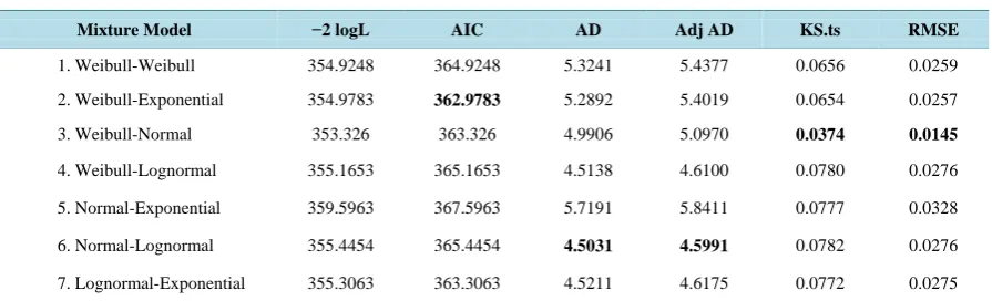
OALibJ | DOI:10.4236/oalib.1101815 5 September 2015 | Volume 2 | e1815 different seven mixture models are estimated for Windshield failure data. The results are displayed in Table 2.

Here, the Weibull-Exponential mixture model contains the smallest AIC value 362.9783, the Normal-Log- normal mixture model contain the smallest value of AD and Adjusted AD test statistics and the Weibull-Normal mixture model contains the smallest value of KS.ts and RMSE among all of the seven mixture models. Hence, we can say that, among these mixture models, Weibull-Exponential, Weibull-Normal and Normal-Lognormal mixture models can be selected as the best three models according to the value of AIC, AD, Adj AD, RMSE and Kolmogrov-Smirnov test statistic, respectively for Windshield failure data.

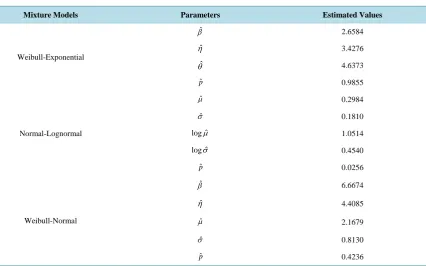
Now, the parameters of Weibull-Exponential, Normal-Lognormal and Weibull-Normal mixture models, esti-mated by applying ML method are displayed in Table 3.

5.

Result Discussion

Murthy et al. [1] assumed that the 2-fold Weibull mixture model fits best for the Windshield data. We have es-timated the CDF and R(t) of 2-fold Weibull mixture model using K-M and ML estimating methods, respectively. The CDF and R(t) are also estimated by using WPP plot [1]. Figure 1 represents the reliability function, to see either the WPP plot or the ML method gives the best result for the data set.

Here, we observe that, the reliability function obtained from the MLE is closer to the Kaplan-Meier estimate than that of the reliability function obtained from the WPP plot. So, we may say that, the maximum likelihood estimate procedure is much better than Weibull probability paper (WPP) plot procedure.

[image:5.595.185.442.367.534.2]

The CDF of Weibull-Exponential, Normal-Lognormal and Weibull-Normal mixture models, using K-M and ML estimating methods are estimated and displayed the results in Figure 2 to identify the model that fits best for the data set.

Figure 1.Comparison of reliability functions of 2-fold Weibull mixture model based on Kaplan-Meier estimate, WPP plot and ML method for Windshield data.

Table 2.Results of various model selection criterions.

Mixture Model −2 logL AIC AD Adj AD KS.ts RMSE

1. Weibull-Weibull 354.9248 364.9248 5.3241 5.4377 0.0656 0.0259

2. Weibull-Exponential 354.9783 362.9783 5.2892 5.4019 0.0654 0.0257

3. Weibull-Normal 353.326 363.326 4.9906 5.0970 0.0374 0.0145

4. Weibull-Lognormal 355.1653 365.1653 4.5138 4.6100 0.0780 0.0276

5. Normal-Exponential 359.5963 367.5963 5.7191 5.8411 0.0777 0.0328

6. Normal-Lognormal 355.4454 365.4454 4.5031 4.5991 0.0782 0.0276

7. Lognormal-Exponential 355.3063 363.3063 4.5211 4.6175 0.0772 0.0275

0 1 2 3 4 5

0

.2

0

.4

0

.6

0

.8

1

.0

Comparison of Reliability

t in thousands hours

Re

lia

b

ilit

y

[image:5.595.92.540.584.720.2]

[image:6.595.148.470.99.241.2]

OALibJ | DOI:10.4236/oalib.1101815 6 September 2015 | Volume 2 | e1815 Figure 2. Comparison of CDFs of Weibull-Exponential, Normal-Lognormal and Weibull-Normal mixture models based on Kaplan-Meier and ML estimate for Windshield data.

Table 3. Estimated values of the parameters.

Mixture Models Parameters Estimated Values

Weibull-Exponential

ˆ

β 2.6584

ˆ

η 3.4276

ˆ

θ 4.6373

ˆ

p 0.9855

Normal-Lognormal

ˆ

µ 0.2984

ˆ

σ 0.1810

ˆ

logµ 1.0514

ˆ

logσ 0.4540

ˆ

p 0.0256

Weibull-Normal

ˆ

β 6.6674

ˆ

η 4.4085

ˆ

µ 2.1679

ˆ

σ 0.8130

ˆ

p 0.4236

From the previous figure, we see among the three mixture models the CDF based on Weibull-Normal mixture model belong very closely to the CDF based on the K-M estimate. Hence we may consider the Weibull-Normal model as the best fitted model for the data set.

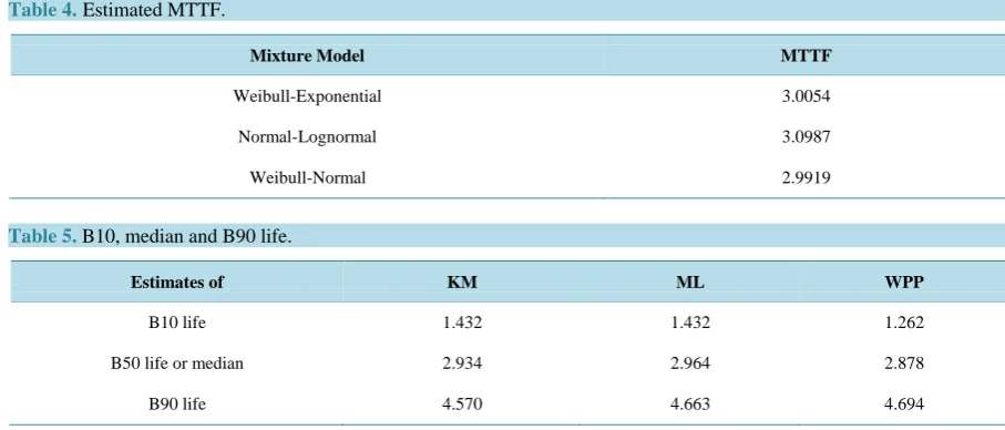
Now, the value of Mean Time to Failure (MTTF) of Weibull-Exponential, Normal-Lognormal & Weibull- Normal Mixture models are given below in Table 4.

The MTTF of the best fitted Weibull-Normal mixture model is 2.9919. And the MTTF value obtained from Weibull-Exponential & Nomal- Lognormal mixture model are 3.0054 & 3.0987, respectively. which are very close to the MTTF of the best fited Weibull-Normal mixture model.

In this article we have also estimated the B10 life, median and B90 life of the CDF based on Kaplan-Meier estimate, ML method and WPP plot for Windshield failure data and displayed the result in Table 5.

[image:6.595.110.537.288.554.2]

[image:7.595.83.537.86.280.2]

OALibJ | DOI:10.4236/oalib.1101815 7 September 2015 | Volume 2 | e1815 Table 4.Estimated MTTF.

Mixture Model MTTF

Weibull-Exponential 3.0054

Normal-Lognormal 3.0987

Weibull-Normal 2.9919

Table 5.B10, median and B90 life.

Estimates of KM ML WPP

B10 life 1.432 1.432 1.262

B50 life or median 2.934 2.964 2.878

B90 life 4.570 4.663 4.694

fail at time 4.570 for K-M procedure, at time 4.663 for MLE and at time 4.694 for WPP plot method. Hence we may say the WPP plot under estimate the B10 life and the median life and over estimate the B90 life compared with K-M and ML methods.

6. Conclusions

Maximum likelihood estimate procedure gives much better fit than Weibull probability paper (WPP) plot pro-cedure. The Weibull-Exponential, Normal-Lognormal & Weibull-Normal mixture models fit well for the Wind-shield failure data, based on the value of AIC, AD, RMSE & Kolmogrov-Smirnov test statistic, respectively. While comparing the CDF values graphically, we found that the Weibull-Normal mixture model belongs very closely to the CDF based on the K-M estimate. The MTTF of the best fitted Weibull-Normal mixture model is 2.9919, which is very close to the other two mixture models. The WPP plot under estimate the B10 life, median life and over estimate the B90 life compared with K-M and ML methods for Windshield failure data.

This article analyzed the product failure data. However, the proposed methods and models are also applicable to analyze lifetime data available in the fields, such as, biostatistics, medical science, bio-informatics, etc. The article considered the first failure data of the product. If, there are repeat failures for any product, application of an approach of modeling repeated failures based on renewal function would be relevant. Finally, further inves-tigation on the properties of the methods and models by simulation study would be useful.

References

[1] Murthy, D.N.P., Xie, M. and Jiang, R. (2004) Weibull Models. John Wiley & Sons, New York.

[2] Karim, M.R. and Suzuki, K. (2005) Analysis of Warranty Claim Data: A Literature Review. International Journal of Quality & Reliability Management, 22, 667-686. http://dx.doi.org/10.1108/02656710510610820

[3] Karim, M.R., Yamamoto, W. and Suzuki, K. (2001) Statistical Analysis of Marginal Count Failure Data. Lifetime Data Analysis, 7, 173-186. http://dx.doi.org/10.1023/A:1011300907152

[4] Meeker, W.Q. and Escobar, L.A. (1998) Statistical Methods for Reliability Data. Wiley, New York.

[5] Murthy, D.N.P. and Djamaludin, I. (2002) New Product Warranty: A Literature Review. International Journal of Pro-duction Economics, 79, 231-260. http://dx.doi.org/10.1016/S0925-5273(02)00153-6

[6] Suzuki, K. (1985a) Non-Parametric Estimation of Lifetime Distribution from a Record of Failures and Follow-Ups. Journal of the American Statistical Association, 80, \68-72.

[7] Suzuki, K., Karim, M.R. and Wang, L. (2001) Statistical Analysis of Reliability Warranty Data. In: Balakrishnan, N. and Rao, C.R., Eds., Handbook of Statistics: Advances in Reliability, Vol. 20, Elsevier Science, 585-609.

http://dx.doi.org/10.1016/s0169-7161(01)20023-6

OALibJ | DOI:10.4236/oalib.1101815 8 September 2015 | Volume 2 | e1815 [9] Kalbfleisch, J.D. and Prentice, R.L. (1980) The Statistical Analysis of Failure Time Data. John Wiley & Sons Inc.,

New York.

[10] Lawless, J.F. (2003) Statistical Methods for Lifetime Data. Wiley, New York.