http://dx.doi.org/10.4236/wjm.2014.45015
How to cite this paper: Shah, A., et al. (2014) Numerical Simulation of Two-Dimensional Dendritic Growth Using Phase- Field Model. World Journal of Mechanics, 4, 128-136. http://dx.doi.org/10.4236/wjm.2014.45015
Numerical Simulation of Two-Dimensional
Dendritic Growth Using Phase-Field Model
Abdullah Shah
1*, Ali Haider
1, Said Karim Shah
21Department of Mathematics, COMSATS Institute of Information Technology, Park Road, Islamabad, Pakistan 2Department of Physics, Abdul Wali Khan University, Mardan, Khyber Pukhtunkhwa, Pakistan
Email: *[email protected]
Received 29 January 2014; revised 26 February 2014; accepted 15 March 2014
Copyright © 2014 by authors and Scientific Research Publishing Inc.
This work is licensed under the Creative Commons Attribution International License (CC BY).
http://creativecommons.org/licenses/by/4.0/
Abstract
In this article, we study the phase-field model of solidification for numerical simulation of den-dritic crystal growth that occurs during the casting of metals and alloys. Phase-field model of soli-dification describes the physics of dendritic growth in any material during the process of under cooling. The numerical procedure in this work is based on finite difference scheme for space and the 4th-order Runge-Kutta method for time discretization. The effect of each physical parameter on the shape and growth of dendritic crystal is studied and visualized in detail.
Keywords
Dendritic Crystal Growth, Phase-Field Model, 4th-Order Runge-Kutta Method
1. Introduction
The study of dendritic crystal growth has become an important aspect in the field of chemical processing, solid state physics and material sciences. The growth of these crystals is a common phenomenon in metals and alloys. The dendrite morphology is also very important in metallurgy. Material properties like volatility, toughness, cor- rosiveness and strength to resist stress depend upon the growth and morphology of these dendrite crystals. The growth of dendrites in any material depends upon the system temperature [1]. During the casting and formation of metals and alloys, these tiny microstructures grow due to the phenomenon of solidification. These tiny micro-structures have a direct impact on the material properties like the quality of a certain material which is influenc- ed by the presence of these microstructures. When metals are casted, dendrites begin to grow due to the process of under-cooling. These dendrites keep on growing until the whole of the liquid phase transforms into solid phase [2]. The study of these dendrites, their size, shape and growth velocity is very important industrially because
they do change the quality of materials. Materials abundant in dendrites are likely to be corrosion and are vulne- rable [1] [3]. This work focuses on the factors responsible for the formation of these patterns and the methods to limit the growth of these solidification microstructures. In the visualization of dendritic structures, the branches and side branches are very important, since the temperature factor greatly limits the growth of these dendrites. We studied numerically the parameters responsible for dendritic growth and tried to explain their effects on the growth. We also explained the fact that, when the temperature is very low, the growth of these dendrites accele-rates. The tip velocity of the side branches is increased by lowering the temperature, whereas the radius or thick- ness of these side branches is small. By increasing the temperature, the growth rate is decreased and side bran- ches grows with less speed while having larger radii [2]. Further increasing the temperature of the system be- yond melting point melts the structure.
2. Phase-Field Model
Phase-field model of solidification were first introduced by Fix [4] and Langer [5] for solving the interfacial problems and to handle the discontinuities involved with the sharp interface model. Phase-field models being numerically simple are very popular in the field of material sciences, solid state physics and electrochemistry in recent years. They are commonly used for the simulation of dendritic growth. This model was first applied for the numerical results of limited diffusion growth by Collins and Levine [6] and by Kobayashi [7] for the study and growth of dendrite. The phase-field model is a mathematical model which explains the physics of dendritic solidification in materials due to undercooling in a natural way. This model has been used extensively to solve the free boundary problems without tracking of the interface at every time step. In Phase-field model, the sharp interface model is replaced by two non-linear equations. The interface between both phases is considered as a diffusion layer with very small thickness [8]. This diffusion layer is given by the Phase-field parameter
ϕ
which is a function of space r and time t. This phase-field or order parameterφ
( )
r,t is also called the level set function which varies from 0 to 1. It has value 0 in the liquid phase and 1 in the solid phase and the inter- mediate value between 0 and 1 gives us the phase transition. This Phase-field parameter distinguishes the solid phase from the liquid phase and the transition layer in between. The problem of locating the position of interface in sharp interface model is covered by this phase-field parameter [9]. The main idea behind the phase-field model is that the jump discontinuity or sharp interface is replaced by a smooth and continuous interface of very small width due to which the singularities involved in the sharp interface model are removed. The main purpose of the phase-field parameterϕ
is to identify the phase by prescribing a value to each phase. Phase-field model of solidification comprises of two parabolic non-linear partial differential equations, the phase-field equation of motion which comprises of the dynamic variable φ( )
r,t and the thermal diffusion equation which consistsof the dimensionless temperature u
( )
r,t with value0 M M T T u T T − = −
. Here, T is the temperature of the system,
M
T is the melting temperature and T0 is the systems initial temperature. The basic equations are:
[ ]
, G t δ ϕ ϕ τ δϕ ∂ = −∂ (2.1)
2 . u u F t t ϕ ∂ = ∇ + ∂ ∂ ∂
(2.2)
[ ]
(
( )
)
2(
( )
)
2 d , 2G ϕ V ϕ δ φ
∇
= +
∫
r r r (2.3)where δ is the interfacial width and V
( )
ϕ is the bulk free energy functional. In this model, we used the dou- ble well free energy functional with prescribed value as:( )
4 1 3 1 2.
4 2 3 4 2
n n
V ϕ =ϕ − − ϕ + − ϕ
(2.4)
This double well free energy functional ensures the growth of the solid phase at the expense of liquid phase. When the free energy of the liquid phase decreases then the liquid phase transforms into solid phase. This free energy functional has two minima, one at ϕ= 0 and the other at ϕ =1 corresponding to the liquid and solid phases respectively. In Equation (2.4), n is a function of dimensionless temperature u with n < 1 2. n> 0
gives the solid phase i.e. ϕ =1 and n~<0 gives the liquid phase ϕ =0, n=0 gives us the phase equili- brium. The prescription chosen for n is
(
)
1 tan
π m
n= β − η T −T
where β and η are the material parameters. T is the actual temperature of the system and Tm is the melting temperature. This prescription of n ensures the growth of the solid phase since it is a difference be- tween the actual temperature T of the system and systems melting temperature Tm. Now most of the phe- nomenon of dendritic growth occurring are anisotropic in nature. In order to introduce anisotropy in Phase-field model of solidification, we assumed the interfacial width δ as a function of angle θ i.e.
δ δ θ
=( )
, whereθ is the angle between the x-axis and ∇ϕ. This angle is in normal direction to the interface and it gives the direction of the interface [11]. For isotropic case this interfacial width δ is constant. The function of interfacial width for the anisotropic case is
( )
(
1 cos(
a0(
0)
)
)
δ θ =δ +µ θ θ−
where µ is the modulation of interfacial width, θ0 is the orientation of the anisotropy axis. Changing the value of θ0 changes the orientation of the dendrite. a0 is the anisotropic mode number, which gives us the shape of the dendrites (for octagonal dendritic structure, we choose a0 =8). Anisotropy in the phase-field model is responsible for the development of side branches of dendrites. Equation (2.2) is the basic time depen-
dent heat equation or the thermal diffusion equation with an extra term F t
ϕ ∂
∂ called the source term, which
accounts for the liberation of latent heat at the interface and maintains the energy balance between both phases. These equations are in their dimensionless units. The final phase-field equations in two dimensions are:
(
)
(
( )
)
( )
2 2 2= 1 1 2 n u ,
t x y y x
ϕ ϕ ϕ
τ∂ ϕ −ϕ ϕ− + − ∂ δδ′∂ + ∂ δδ′∂ + ∇ δ ⋅∇ + ∇ϕ δ ϕ
∂ ∂ ∂ ∂ ∂ (2.5)
2 , u u F t t ϕ ∂ = ∇ + ∂ ∂ ∂
(2.6)
The solution of the phase-field Equation (2.5) describes the shape, motion and location of the diffusion layer, while the solution of the thermal-diffusion Equation (2.6) gives the temperature of the interfacial layer.
3. Numerical Method and Results
For space discretization, we applied the method of finite difference (central difference scheme) and for time discretization, we applied the 4th-order Runge-Kutta method. The Laplacians ∇2
ϕ
and 2u
δ
, melting temperature TM , time t, latent heat F and mode number of anisotropy a0 are studied separately and their effects on the dendrite are visualized. Numerical results for both phase-field ϕ and temperature u are presented here for different values of time. We focused in this study, on the measures of controlling the growth of dendrites. We also presented here the effect of each parameter on the tip velocity and tip radius of side branches. Since the side branches in dendritic growth are very important from industrial point of view. Their presence directly affects the quality of material and they normally occur due to the presence of impurities in the material. Therefore, we also focused on the effect of each parameter on the side branches.3.1. Effect of Relaxation Time on Dendrite
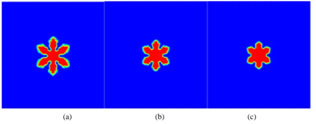
In Figures 1(a)-(c), results are compared using different values of
τ
. For ∆ = ∆ =x y 0.03 and ∆ =t 0.0001, we have compared the dendritic growth for τ =0.0003, 0.0004 and 0.0005, inside square domain of size[
0, 215] [
× 0, 215]
with anisotropy a0=6 and at time t=0.1. The graphs clearly shows that for small values of relaxation time i.e., for τ =0.0003, the growth process is much faster as compared to τ =0.0004 and0.0005. This is in agreement to the fact that, for small values of relaxation time
τ
, the atoms takes less time to retain their equilibrium position and undergo the process of nucleation, while for large values of relaxation time the equilibrium state is retained lately. Relaxation time has an indirect effect on the tip velocity and tip radius of side branches. Note that in Figures 1(a)-(c) both tip velocity and tip radius of side branches decreases as the re- laxation time is increased from τ = 0.0003 to 0.0005.3.2. Effect of Orientation Angle on Dendrite
The angle θ0 is the orientation of anisotropy axis and changing the value of θ0 brings changes in the ori- entation of dendritic crystal. With anisotropy a0=6, Figure 2(a)and Figure 2(b)shows the rotational effect of crystal at an angle of 90˚ which is due to the change in the value of orientation angle θ0 from 1.57 to 0.05
respectively. It also shows that θ0 changes only the orientation of the crystal keeping the shape and growth of dendrite unaffected.
[image:4.595.141.460.408.533.2](a) (b) (c)
Figure 1. Crystal growth at (a) τ=0.0003; (b) τ=0.0004; and (c) τ=0.0005.
[image:4.595.169.431.560.704.2](a) (b)
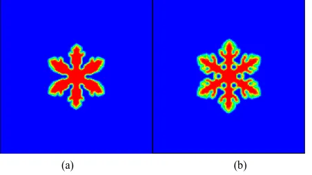
3.3. Effect of Interfacial Width on Dendrite
In this subsection, for the same values of step size, ∆t and a0, we computed the problem for two different 0.01
δ= and 0.011 for time t=0.12 as shown in Figure 3(a) and Figure 3(b). We observed that when the in- terfacial width δ is slightly increased from 0.01 to 0.011 respectively, the tip velocity and tip radius of side branches also increased. Note that for interfacial width δ =0 the growth of the crystal almost ceases (the me- thod diverges).
3.4. Effect of Melting Temperature on Dendrite
In this subsection, we gave the numerical simulation for different values of melting temperature TM for phase- field distribution ϕ. Using square domain of size
[
0, 215] [
× 0, 215]
with ∆ =x 0.03, ∆ =t 0.0002, a0 =6, and latent heat F=2.0, we compared the results for TM =1.0, 1.1 and 1.2 at time t=0.2. Figures 4(a)-(c)shows the effect of melting temperature TM on the size, shape and growth of dendrite for phase-field ϕ dis- tribution. Since the dimensionless temperature u is given by
0 M
M
T T
u
T T
− =
−
where T is the temperature of the system, TM is the melting temperature and T0 is the system’s initial temperature with value T0 =0. As the value of TM is increased from 1.0 to 1.2, the dimensionless temperature
u decreases. Therefore, the growth process accelerates by increasing the value of TM (Figures 4(a)-(c)). Note that melting temperature TM has a direct effect on the growth and shape of dendrite. It is also clear from
Figures 4(a)-(c) that increasing the melting temperature TM , increases the tip velocity of side branches while the tip radius has an inverse effect. When TM is increased, the dimensionless temperature u~ decreases and the tip radius of side branches decreases. When the dimensionless temperature u~ is very low the growth of these dendrites accelerates, the tip velocity of the side branches is increased by lowering the temperature, where- as the radius or thickness of these side branches is small. By increasing the temperature, the growth rate is de- creased, side branches grow with less speed while have larger radii. Further increasing the temperature of the system beyond melting point melts the structure.
[image:5.595.188.414.431.558.2](a) (b)
Figure 3. Crystal growth at (a) δ=0.01; (b) δ=0.011.
[image:5.595.147.451.585.707.2](a) (b) (c)
3.5. Effect of Anisotropy on Dendrite
Anisotropy has a direct effect on the shape of dendritic crystal. In Figure 5, we presented the tetragonal shape of dendrite using mode number of anisotropy a0 =4, on square mesh of size
[
0, 215] [
× 0, 215]
with ∆ =t 0.0001, latent heat F =1.8, relaxation time τ=0.0003, orientation angle θ =0 1.57, interfacial widthδ
=0.01 and0.03
x y
∆ = ∆ = at time t=0.2 both for phase-field and temperature values respectively. We now present the
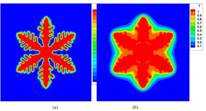
hexagonal shape of dendrite in Figure 6, by increasing the mode number of anisotropy a0 =6, on square mesh of size
[
0, 215] [
× 0, 215]
with ∆ =t 0.0001, latent heat F=1.8, relaxation time τ =0.0003, orientation angle θ =0 1.57, interfacial widthδ
=0.01 and ∆ = ∆ =x y 0.03, both for phase-field and temperature values respectively at time t=0.2. Note that anisotropy has a direct affect on the side branches. As clear fromFigures 5-7, when anisotropy is increased from a0=4 to a0=6, the side branches appear around the crystal. Moreover the tip velocity and tip radius of side branches is also increased when anisotropy is changed from 4 to 6. We now give the octagonal shape of dendrite by using mode number of anisotropy a0 =8 under the same values of physical parameters at time t=0.2. In Figure 7, we have simulated the results for both phase-field and temperature distribution respectively. The anisotropic mode number a0 tells us about the presence of im- purities in a material. Materials abundant in impurities have large anisotropic mode numbers and therefore a large amount of side branches grow around the dendritic crystal with larger radii.
3.6. Effect of Latent Heat on Dendrite
The whole growth process of the dendrite depends mainly upon latent heat F. This auxiliary parameter is the most important physical quantity of the phase-field model. It accounts for the liberation of heat from the solidifi-
[image:6.595.157.440.348.499.2](a) (b)
Figure 5. Dendritic growth for anisotropy a0=4. (a) (Phase-field distribu- tion); (b) (temperature distribution).
[image:6.595.156.441.539.693.2](a) (b)
(a) (b)
Figure 7. Dendritic growth for anisotropy a0=8. (a) (phase-field distribution); (b) (temper- ature distribution).
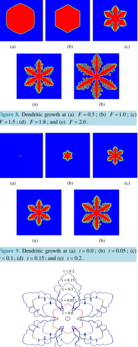
cation front (diffusion layer). Large values of latent heat F accounts for the evacuation of heat from the inter- facial region in a great amount. Therefore, the growth of dendrite is directly proportional to the value of latent heat F. For small values of F the growth process is slow, as less amount of heat evacuates from the diffusion layer and hence the solidification process is slow. Latent heat F is the main parameter which triggers the so- lidification process. Figures 8(a)-(e) shows the dendritic growth for latent heat F=0.5, 1.0, 1.5, 1.8 and 2.0, inside square domain of size
[
0, 215] [
× 0, 215]
with ∆ =t 0.0002, relaxation time τ =0.0003, orientation angle θ =0 1.57, interfacial widthδ
=0.01, mode number of anisotropy a0 =6 and ∆ = ∆ =x y 0.03 res- pectively at time t=0.1. Figures 8(a)-(e)clearly shows that the shape of dendrite depends upon the latent heat F, for large values of F the branches and side branches form around the dendritic crystal. Latent heat F has a di- rect effect on the tip radius and tip velocity of side branches. As latent heat F increases from 0.5 to 2.0, the tip radius and tip velocity of side branches also increases. Therefore, in order to limit the growth of side branches, latent heat F should be taken small.3.7. Effect of Time on Dendrite
Time has a direct effect on the growth as well as on the shape of dendritic crystal. Figures 9(a)-(e) shows the effect of time on the dendritic growth for t=0.0, 0.05, 0.1, 0.15 and 0.2 respectively with relaxation time
0.0003
τ = , orientation angle θ =0 1.57, interfacial width δ =0.01, mode number of anisotropy a0 =6, 0.03
x y
∆ = ∆ = , ∆ =t 0.0001 and latent heat F=1.8. Figure 9 clearly shows the effect of time on the growth and shape of dendrites. At time t=0.0, we get the central nucleus while for large values of time the growth process accelerates along with the shape. The branches and side branches form around the solid grain for large values of time. In Figure 10, we have given contour plot of dendritic growth for time t=0.0, 0.05, 0.1, 0.15 and 0.2 respectively. It also shows the acceleration of growth phenomenon with the passage of time. Clearly the interfacial velocity is a function of time. The tip radius and tip velocity of side branches also increases by increasing the time.
4. Conclusion
(a) (b) (c)
(a) (b)
Figure 8. Dendritic growth at (a) F=0.5; (b) F=1.0; (c) 1.5
F= ; (d) F=1.8; and (e) F=2.0.
(a) (b) (c)
[image:8.595.188.413.92.657.2](a) (b)
Figure 9. Dendritic growth at (a) t=0.0; (b) t=0.05; (c) 0.1
t= ; (d) t=0.15; and (e) t=0.2.
Figure 10. Dendritic growth at t=0.0, t=0.05, 0.1
dendritic crystal are simulated and presented. Effects of these parameters on the tip velocity and tip radius of side branches are also presented.
References
[1] Glicksman, M.E. and Marsh, S.P. (1993) Handbook of Crystal Growth. North-Holland, Amsterdam, 1075-1080.
[2] Boettinger, W.J., Coriell, S.R., Greer, A.L., Karma, A., Kurz, W., Rappaz, M. and Trivedi, R. (2000) Solidification Mi- crostructures: Recent Developments, Future Directions. Acta Materialia, 48, 43-70.
http://dx.doi.org/10.1016/S1359-6454(99)00287-6
[3] Cahn, J.W. (1967) Crystal Growth. Pergamon Press, Oxford, 681-690.
[4] Fix, G.J. (1983) Free Boundary Problems. Boston, 115-135.
[5] Langer, J.S. (1980) Instabilities and Pattern Formation in Crystal Growth. Reviews of Modern Physics, 52, 1-28.
http://dx.doi.org/10.1103/RevModPhys.52.1
[6] Collins, J.B. and Levine, H. (1985) Diffuse Interface Model of Diffusion-Limited Crystal Growth. Physical Review B,
31, 160-195. http://dx.doi.org/10.1103/PhysRevB.31.6119
[7] Kobayashi, R. (1993) Modeling and Numerical Simulations of Dendritic Crystal Growth. Physica D, 63, 410-423.
http://dx.doi.org/10.1016/0167-2789(93)90120-P
[8] Ying, X., McDonough, J.M. and Tagavi, K.A. (2006) A Numerical Procedure for Solving 2D Phase-Field Model Pro- blems, Journal of Computational Physics, 218, 770-793. http://dx.doi.org/10.1016/j.jcp.2006.03.007
[9] Wheeler, A.A., Murray, B.T. and Schaefer, R.J. (1993) Computation of Dendrites Using a Phase-Field Model. Physica D, 66, 243-262. http://dx.doi.org/10.1016/0167-2789(93)90242-S
[10] Biben, T. (2005) Phase-Field Models for Free-Boundary Problems. European Journal of Physics, 26, 47-55.
http://dx.doi.org/10.1088/0143-0807/26/5/S06