Three Dimensional Finite Element Analysis of Wire
Drawing Process
Abdul Kareem F. Hassan
*, Alyaa S. Hashim
Department of Mechanical Engineering, University of Basrah, Iraq
Copyright © 2015 Horizon Research Publishing All rights reserved.
Abstract
This work aims to analytically and numericallystudy the parameters affecting on the wire drawing process using a 3D finite element model and the effect of these parameters on drawing force. Three-dimensional finite element model using DEFORM-3D V6.1 was built to simulate this process. AL-1100 wire was drawn through a conical die with semi-die angle
(
α = 6° , 8° , 8.5° , 9° , 9.5° , 10°,, 15° ), reduction ratio ( r = 0.1 , 0.15 , 0.2 , 0.25 , 0.3), friction coefficient ( µ = 0.1 , 0.08 , 0.075 , 0.07 , 0.065 , 0.06 , 0.05), bearing length ( BL= 0.5 , 0.75 , 1 , 1.25 , 1.6 ) mm, drawing velocity ( 5000, 7500, 10000, 12500, 15000, 17500, 20000)mm/sec. were taken in this study. Many simulations with different parameters were taken to capture the optimum die angle. The results show that the optimum die angle depends on reduction in area (α= 9.5°, 9.5°, 9.5°,10°, 10°) for reduction in area (r= 0.1, 0.15, 0.2, 0.25, 0.3). The drawing force estimated from finite element results was compared with that of analytical results and found in line with maximum error percentage of 4%. The results of finite element model were analyzed statistically using SPSS software in order to find the relationship between the above factors and drawing force.Keywords
Wire Drawing Process, Slab Method, FiniteElement Method
1. Introduction
Wire drawing process is one of the most used metal forming processes within the industrial field [1]. The process consists of changing and reducing the cross-section area of a wire by pulling it through a conical die, creating a long product with a constant cross-section that has an excellent surface finish, closely controlled dimensions, and improved mechanical properties such as strength and hardness [2]. Materials traditionally used in this kind of manufacturing processes are aluminum, copper alloys and steel.
There have been many investigator who studied the wire drawing process. Rubio et al.[1] studied the main variant of drawing process: the homogeneous deformation of the
material and the friction between the work-piece material and the die-interfaces to estimate the necessary force to carry out the process, by different methods. Wire drawing and plate drawing have been modeled and simulated by means of the slab method (SM) and finite element method (FEM). The solutions comparison confirms that FEM is a more accurate method than SM because the obtained results with it are nearer to the real results. FEM provides very intuitive simulations in which the forward tension can be seen not only at the die exit but also in the deformation zone. SM underestimates the drawing stress value to carry out a certain process, since it only accounts the homogeneous deformation and friction. SM forward tension curves only are similar to experimental and FEM ones for low reductions carried out in dies with low semi-angles and under low friction conditions. Kabayama et al. [3] studied the influence of die geometry in determining the surface and mechanical properties of drawn wires, and consequently, their application. Annealed electrolytic copper wire, with 0.5mm original diameter was reduced by 19% in dies with 2α =10˚ and 18˚ and BL=35 and 50%. The best experimental results were then studied by the finite element method to simulate residual stress distribution. The experimental results show that the friction coefficient decreases as the wire drawing speed increases, and that small 2α and BL values bring about the most favorable wiredrawing conditions.
5.50mm from steel grade 0.46% carbon and 0.71% carbon were drawn to 1.35mm in 13 draws and two speeds 8m/sec and 25m/sec. After each draw, the following properties were determined; tensile strength (Ts), temperature (T), number of twists (Nt), number of bends (Nb). A large drop in the number of twists has been observed for final wire because of increased draw speed. The drawing speed depends on wire material as well as reduction in area for high speed. However, there is also an advantage as the wire surface is much smoother after drawing at high speed than at low speed. The results show the increase of speed caused the increase of tensile strength and causes rise in temperature. Cetinarslan [6] studied the influences of some parameters like deformation (total reduction) ratio and drawing speed on cold drawing of ferrous wires. Wire drawing method is applied to C45, C46, C65 and C70 materials for different deformation ratios and different drawing velocities. Subsequently, these process influences are considered by means of tensile tests. With these investigations, it can simply observed that the deformation ratio and drawing speed parameters clearly affect tensile of ferrous materials. In addition to these observations, from the results of experiments the tensile strength increases gradually as the drawing speed increases and as the reduction ratio goes up. It is a known fact that increasing reduction or deformation ratio causes an increase in strain hardening and as a result yield stress of materials also increases. Strain hardening (work-hardening) is the process of making a metal harder and stronger through plastic deformation. Carbon content also effects tensile strength of steel wires but this effect is not as much as the drawing speed and reduction ratio. Cetinarslan and Güzey [7] studied the influence of drawing-process parameters such as reduction (deformation) ratio and drawing velocity on the tensile properties of various low-carbon cold-malleable steels wires.
The obtained results have shown that the yield strength and ultimate tensile strength increase, while the elongation at rupture decreases for all the steels when the reduction ratio is increased. The drawing velocity has a significant effect on the tensile properties (the yield and the ultimate tensile strength) of low-carbon steel wires. A high drawing velocity causes high strength properties. The values of elongation at rupture also decrease as the drawing velocity increases.
The aim of this work is to find relationships between drawing force and semi-die angle, bearing length and reduction in area. First step is the verification of the finite element model, which can be achieved through the comparison of the finite element results with previous analytical models which can be found in many literature. The second step is the analyzing of the finite element results using the proper statistical techniques.
2. Theoretical Background
Using slab method the plastically deformation zone has been modeled as shown in Figure (1). The total drawing
[image:2.595.313.552.155.272.2]stress is the result of the influence of three components (ideal or homogeneous deformation required to reduce the cross section, frictional deformation required to overcome frictional resistance, and redundant deformation required to change the flow direction). Calculation of the drawing stress can be classified into three categories:
Figure 1. A wide strip is being drawn through a frictionless die with a total
included angle of 2α [8].
For an ideal plastic deformation the drawing stress can be calculated by [9],
𝜎𝜎𝑎𝑎= 𝜎𝜎°ln1−𝑟𝑟1 (1) (the frictional and redundant deformation are neglected in equation (1))
Since 𝜎𝜎°= 𝐾𝐾 𝜖𝜖 𝑛𝑛
𝑛𝑛+1 (2) And ∈ = ln1−𝑟𝑟1
where:
𝜎𝜎° = average flow stress for material r = is the deformation ratio i.e. 𝑟𝑟 = 1 − ℎ𝑎𝑎
ℎ𝑏𝑏 K = strength coefficient
n= strain-hardening exponent
∈
= true strain [image:2.595.332.534.543.696.2]where K and n can be found in such literature [10] and shown in Table (1).
Table 1. Value of K and n [10]
Material K (Mpa) n
Al 1100 180 0.2
deformations were taken without the effect the redundant deformation, the drawing stress can be written as [1].
𝜎𝜎𝑎𝑎= 𝜎𝜎°�1+𝐵𝐵𝐵𝐵 � � 1 − ( 1 − 𝑟𝑟 )𝐵𝐵 � (3) where 𝐵𝐵 = 𝜇𝜇 cot 𝛼𝛼 and 𝛼𝛼 is the semi die angle.
For wire drawing process conducted with conical dies the equation (3) can be expressed as [9],
Since 𝑟𝑟 = 1 − ( 𝐷𝐷𝑎𝑎
𝐷𝐷𝑏𝑏 ) 2 (4)
where:
𝐷𝐷𝑏𝑏= wire diameter before drawing
𝐷𝐷𝑎𝑎 = wire diameter after drawing
Subtitling in equation (3), one can get [11]:
𝜎𝜎𝑎𝑎= 𝜎𝜎°1+𝐵𝐵𝐵𝐵 � 1 − �𝐷𝐷𝐷𝐷𝑎𝑎
𝑏𝑏� 2𝐵𝐵� (5)
The redundant deformation has adverse effects on wire properties in addition to increasing the stress needed for drawing. One consequence is that mechanical properties will not be homogeneous across the wire section because redundant deformation is concentrated close to the wire surface, higher levels of strain hardening will result in the surface and near layers and will be greater than the strain that results from cross section reduction. The redundant deformation is influences of residual stress in drawn wire. As the semi-die angle is increased the deformation between the surface and centerline also increases. This leads to progressively higher tensile stress at surface and compression stresses at the core. The value of redundant deformation depends on the value of semi-die angle and reduction ratio which represent the effect of geometry of the die and can be referred as delta factor (Δ) [12],
∆ = 𝛼𝛼𝑟𝑟� 1 +� 1 − 𝑟𝑟 �1 2⁄ �2 (6)
The redundant deformation factor (
𝜑𝜑
) is related by the parameter Δ [12],𝜑𝜑= ∆6+ 1 (7)
Note that redundant factor increases substantially as Δ increases.
The finial total drawing stress can be determined after knowing the values of the three parts from the following equation [11],
𝜎𝜎𝑎𝑎= 𝜑𝜑 𝜎𝜎°1+𝐵𝐵𝐵𝐵 � 1 − �𝐷𝐷𝐷𝐷𝑎𝑎𝑏𝑏� 2𝐵𝐵� (8)
3. Materials and Die Geometry
Aluminum alloys 1100 is used in many important applications due to good thermal and electrical conductivity and corrosion resistance, excellent formability, light weight compared to steel and copper, high efficiency and lower cost. Aluminum - 1100 contains 99% of aluminum in composition. The properties and chemical composition of wire materials are shown in Table (2)[13]. This alloy is soft
and causing a lot of problems during the drawing process due to the inappropriate selection of the die design and velocity.
Before using Deform-3D code it is necessary to start AutoCAD 2012 which used to design the die and wire at the standard dimensions of drawing die (According to practical die standard ), as shown in Table (3) [14].
In order to determine the drawing force a wire made of Aluminum-1100, with 3mm of original diameter, was carried out on a single die with constant drawing velocity 5000 mm/sec. Different values of the reduction in area ( r = 10, 15, 20, 25, 30 )% and the final diameter of the wire (2.84, 2.76, 2.68, 2.59, 2.5)mm, respectively. These cases were run for different values of semi-die angle (α = 6, 8, 8.5, 9, 9.5, 10, 15)˚and the friction coefficient(µ = 0.1,0.08,0.075,0.07, 0.065, 0.06, 0.05) respectively.
Table 2. Chemical composition and Mechanical properties for Al-1100 [13]
Chemical composition
Other Element (Fe,Mg,Ti,Cr,Bi,
Pb) Zn
Si Mn Cu
Al
Total Each
0.15% 0.05%
0.10% 0.95Si
+ Fe 0.05
% 0.05-0.20
% 99.0
%
Mechanical properties Specified diameter 3.1496mm and under Tensile strength , Mpa
Max. Min.
106.868765 75.842349
Table 3. Dimension of drawing die [14]. Die
12 mm Outer Diameter
10 mm Outer height
10˚
Exit angle
1 mm Bearing length
Wire
3 mm Original diameter
2.84, 2.76, 2.68, 2.59 and 2.5 Final diameter
150 mm Length
4. Finite Element Modeling of Wire
Drawing
In this study the code DEFORM-3D V6.1 is used to perform the finite element analysis of wire drawing process. This software is specifically designed to analyze bulk plastic deformation, and is especially suited for the present analysis. It takes advantage of the fact that plastic deformation is usually highly localized. It assigns rigid elements to the regions of the part that are not deforming, thereby reducing the number of calculations performed at each step of the simulation. It also updates nodal coordinates using a high order scheme [15].
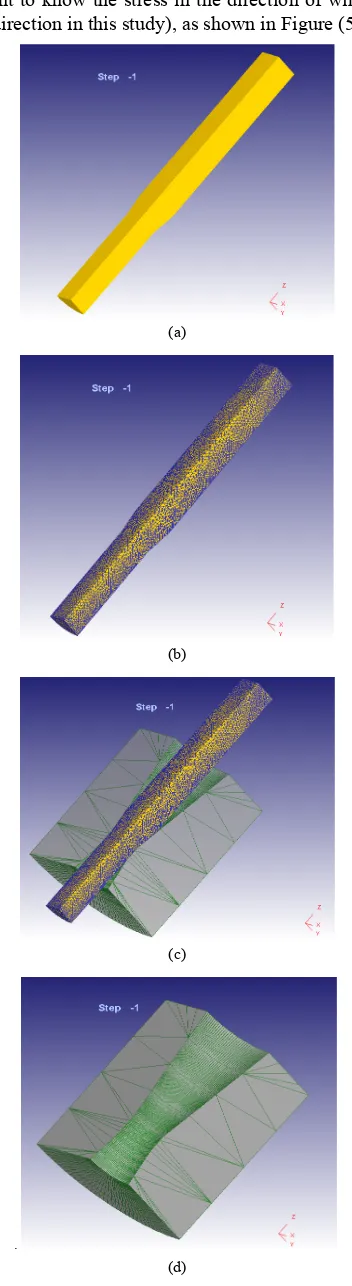
elements on the surface of that wire, while the volume mesh generates elements inside the volume of the wire plus the outer surface. Simulations were performed to evaluate how many elements along the radial direction were necessary to obtain convergence of the drawing stress data. In Deform-3D code, there are two types of elements tetrahedral mesh and brick mesh. In this work the tetrahedral mesh of selected in the mesh generation of the wire because it is suitable for this kind of forming process [16].
Due to symmetry only one quarter of die and wire were used in this simulation. Figure (3-a) shows the wire geometry. After making several attempts it was found that the appropriate number of element is (44421) while the number of nodes are ( 133263 ), as shown in Figure (3-b).Since the die, as shown in Figure (3-c), is rigid which does not deform during the drawing process so it does not need meshing and does not move in any direction, Adjustments to the die profile were limited to the approach angle, inner diameter and bearing length. Finally, the wire takes position within the die shown in Figure (3-d). as well as defining of the friction coefficient between interface of the die and wire.
4.1. Applying the Drawing Velocity and Boundary Conditions
After building the model, the following step was to apply velocity to the structure in preparation for solution. In order to properly model structures behavior, it is necessary to apply velocity with respect to a specified time interval. Unlike most implicit analysis, all resulting stress in an explicit analysis must be time- dependent in nature.
The following are the parts and the boundary conditions applied to them:
(i). The Die Part
Since the die is rigid which does not contain elements to the regions of the part and does not deform, the boundary conditions applied are: zero displacement in all directions and zero rotations in all directions.
(ii). The Wire Part
Since the wire is plastic which is the only part that suffers deforming during the drawing process. In this process a small part of the wire extended in to the die, the boundary condition for the wire part represented by signing the drawing velocity on the small part of the wire as shown in Figure (4) , the boundary conditions are : zero velocity in the x and y directions and 5000 mm/sec. on the z-direction .
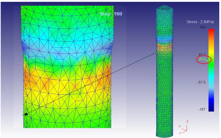
Finally, the number of simulation steps are selected 160 steps ( after a number of attempts ) to find out the number of steps required for drawing process before the wire arrivaed the end of bearing region. The step increment to save is selected per 10 steps, and the selected time drawing process was small in order to reduce the number of steps.
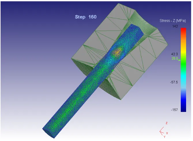
After the completion of the model building and applying the boundary condition, the case can be solved using the simulator utility. The post-processor shows the results of the simulated case. In the wire drawing process, it is most
important to know the stress in the direction of wire center line (z direction in this study), as shown in Figure (5)
(a)
(b)
(c)
.
[image:4.595.343.519.83.726.2](d)
Figure 4. Application of velocity boundary condition on z-direction.
Figure 5. The value of total z-stress at r%=0.1 , α=9.5 and µ=0.065
5. Results and Discussion
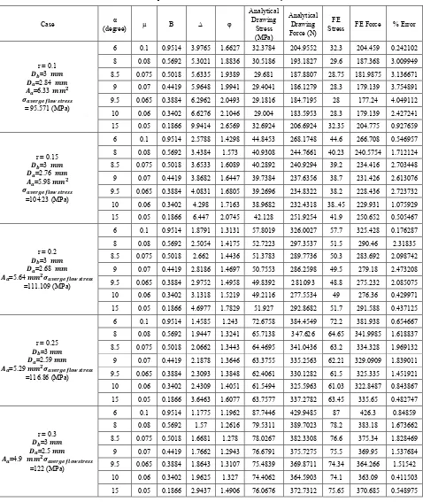
In this section, the effect of the change in the semi-die angle on the values of drawing stresses resulting during the drawing process was discussed. These stresses could be analyzed by identifying of the types of deformation in the wire (homogeneous, frictional and redundant), using the equations in the theory of wire drawing section, as shown in Table (4).
During the different steps in the finite element results, there will be stresses with different sings and magnitude. The z-stress, created by material flow, is one of the important types. The z-stress distribution on cross and longitudinal sections in the wire must be in equilibrium. The stress analyses can be conducted to determine total stress variation in the material during the wire drawing process. These analyses are very important in the wire drawing process
optimization considering low possible contact force. The total z-stress value is found near the surface layer at the wire exit from the die [17].
Table (4) explains the comparison between the analytical results and finite element results, with the percentage error in the two values. The percentage error was calculated using the following equation.
𝐸𝐸𝑟𝑟𝑟𝑟𝐸𝐸𝑟𝑟 % = �𝜎𝜎𝐴𝐴𝑛𝑛𝑎𝑎𝐴𝐴𝐴𝐴𝐴𝐴𝐴𝐴𝐴𝐴𝑎𝑎𝐴𝐴− 𝜎𝜎𝐹𝐹𝐸𝐸
𝜎𝜎𝐴𝐴𝑛𝑛𝑎𝑎𝐴𝐴𝐴𝐴𝐴𝐴𝐴𝐴𝐴𝐴𝑎𝑎𝐴𝐴 � × 100 % (9)
Where:
𝜎𝜎𝐴𝐴𝑛𝑛𝑎𝑎𝐴𝐴𝐴𝐴𝐴𝐴𝐴𝐴𝐴𝐴𝑎𝑎𝐴𝐴= Analytical Drawing Stress,
𝜎𝜎𝐹𝐹𝐹𝐹 = Finite Element Drawing Stress.
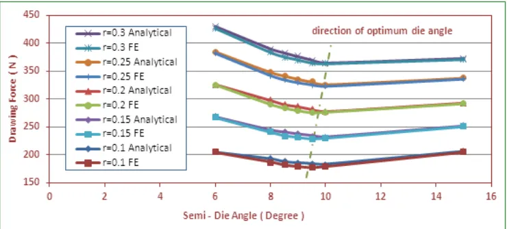
[image:5.595.138.473.277.522.2]Figure 6. Effect of semi- die angle on drawing force at different Reduction in Area. Figure (6) shows the effect of semi-die angle on the
drawing force at different deformation ratio. For r=0.1 and α=6˚, it can be seen that the value of drawing force has a large value [204.9552 N as shown in Table 4] and this can be attributed to the high frictional stress concerning small die angle [𝜎𝜎𝑓𝑓𝑟𝑟𝐴𝐴𝐴𝐴𝐴𝐴𝐴𝐴𝑓𝑓𝑛𝑛𝑎𝑎𝐴𝐴=9.3438 Mpa for α=6˚].
The value of drawing force then gradually decreases as the die angle increased until the die angle reaches an optimum value [α approximately equal to 10˚]. After that the drawing force will increase because the redundant stress increased with [drawing stress increased from 29.004 MPa at α=10˚ to 32.6924 MPa at α=15˚] increasing die angle [increase from 15.2225 MPa at α=10˚ to 20.3877 MPa at α=15˚].
Same behavior was observed for other drawing ratios. Increasing the drawing ratio will shift the curve to the top.
The purpose of constructing these curves to get the optimum die angles (9.5, 9.5, 9.5, 10˚ and 10˚) for each value of reduction in area (0.1, 0.15, 0.2, 0.25 and 0.3) respectively. An optimum die angle is the angle from which minimizes the value of both friction and redundant deformation as well as getting less the drawing force with good wire specification (hardness, high strength, less ductile).
5.1. Effect of Bearing Length on Drawing Force
In wire drawing process many changes occur during the passing of wire through the die, see Figure (7-a).(region I): in this region the existence of the redundant deformation is shown which occurs due to coming together with the wire and the die angle. The redundant deformation is previously noted that it increases with the die angle. In the approach region (region II), radial compression increases for all nodes. The wire surface is more compressed than other regions due to the wire drawing die compression force on the outer layer of the wire .In the bearing region (region III), a change from
[image:6.595.316.548.365.493.2]compression stress to drawing stress occurs that increasing the length of this region causes an increase in residual stress values .The residual stress found in exit region (region IV) shows its importance for the equilibrium of the compression and drawing stresses. The deformation occurs on several outer layers of the wire caused by the wire drawing die geometry, shown in Figure (7) [b,c].
Figure 7-a. The parts of a wire drawing die [18].
In order to observe the effect of bearing length on the drawing force several values of bearing length ( 0.5, 0.75, 1, 1.25 and 1.6 )mm with constant drawing ratio (r=0.1), and different die angles (α=6˚, 10˚, and 15˚) were taken in this study. It was found that increasing the bearing length will increase the drawing force and the minimum drawing force was observed when the value of α is optimum, as shown in Figure (7-b). These results agree with the results of Kabayama et al. [3].
Table 4. The comparison between the finite element and analytical results % Error FE Force FE Stress Analytical Drawing Force (N) Analytical Drawing Stress (MPa) φ ∆ B µ α (degree) Case 0.242102 204.459 32.3 204.9552 32.3784 1.6627 3.9765 0.9514 0.1 6
r = 0.1
𝑫𝑫𝒃𝒃=3 𝒎𝒎𝒎𝒎
𝑫𝑫𝒂𝒂=2.84 𝒎𝒎𝒎𝒎
𝑨𝑨𝒂𝒂=6.33 𝒎𝒎𝒎𝒎𝟐𝟐
𝝈𝝈𝒂𝒂𝒂𝒂𝒂𝒂𝒂𝒂𝒂𝒂𝒂𝒂 𝒇𝒇𝒇𝒇𝒇𝒇𝒇𝒇 𝒔𝒔𝒔𝒔𝒂𝒂𝒂𝒂𝒔𝒔𝒔𝒔 = 95.571 (MPa)
3.009949 187.368 29.6 193.1827 30.5186 1.8836 5.3021 0.5692 0.08 8 3.136671 181.9875 28.75 187.8807 29.681 1.9389 5.6335 0.5018 0.075 8.5 3.754891 179.139 28.3 186.1279 29.4041 1.9941 5.9648 0.4419 0.07 9 4.049112 177.24 28 184.7195 29.1816 2.0493 6.2962 0.3884 0.065 9.5 2.427241 179.139 28.3 183.5953 29.004 2.1046 6.6276 0.3402 0.06 10 0.927659 204.775 32.35 206.6924 32.6924 2.6569 9.9414 0.1866 0.05 15 0.546957 266.708 44.6 268.1748 44.8453 1.4298 2.5788 0.9514 0.1 6
r = 0.15
𝑫𝑫𝒃𝒃=3 𝒎𝒎𝒎𝒎
𝑫𝑫𝒂𝒂=2.76 𝒎𝒎𝒎𝒎
𝑨𝑨𝒂𝒂=5.98 𝒎𝒎𝒎𝒎𝟐𝟐
𝝈𝝈𝒂𝒂𝒂𝒂𝒂𝒂𝒂𝒂𝒂𝒂𝒂𝒂 𝒇𝒇𝒇𝒇𝒇𝒇𝒇𝒇 𝒔𝒔𝒔𝒔𝒂𝒂𝒂𝒂𝒔𝒔𝒔𝒔 =104.23 (MPa) 1.712124 240.5754 40.23 244.7661 40.9308 1.573 3.4384 0.5692 0.08 8 2.703448 234.416 39.2 240.9294 40.2892 1.6089 3.6533 0.5018 0.075 8.5 2.613076 231.426 38.7 237.6356 39.7384 1.6447 3.8682 0.4419 0.07 9 2.723732 228.436 38.2 234.8322 39.2696 1.6805 4.0831 0.3884 0.065 9.5 1.075929 229.931 38..45 232.4318 38.9682 1.7163 4.298 0.3402 0.06 10 0.505467 250.652 41.9 251.9254 42.128 2.0745 6.447 0.1866 0.05 15 0.176287 325.428 57.7 326.0027 57.8019 1.3131 1.8791 0.9514 0.1 6
r = 0.2
𝑫𝑫𝒃𝒃=3 𝒎𝒎𝒎𝒎
𝑫𝑫𝒂𝒂=2.68 𝒎𝒎𝒎𝒎
𝑨𝑨𝒂𝒂=5.64 𝒎𝒎𝒎𝒎𝟐𝟐𝝈𝝈𝒂𝒂𝒂𝒂𝒂𝒂𝒂𝒂𝒂𝒂𝒂𝒂 𝒇𝒇𝒇𝒇𝒇𝒇𝒇𝒇 𝒔𝒔𝒔𝒔𝒂𝒂𝒂𝒂𝒔𝒔𝒔𝒔 =111.109 (MPa) 2.31835 290.46 51.5 297.3537 52.7223 1.4175 2.5054 0.5692 0.08 8 2.098742 283.692 50.3 289.7736 51.3783 1.4436 2.662 0.5018 0.075 8.5 2.473208 279.18 49.5 286.2598 50.7553 1.4697 2.8186 0.4419 0.07 9 2.085075 275.232 48.8 281.093 49.8392 1.4958 2.9752 0.3884 0.065 9.5 0.429971 276.36 49 277.5534 49.2116 1.5219 3.1318 0.3402 0.06 10 0.437125 291.588 51.7 292.8682 51.927 1.7829 4.6977 0.1866 0.05 15 0.654667 381.938 72.2 384.4549 72.6758 1.243 1.4585 0.9514 0.1 6
r = 0.25
𝑫𝑫𝒃𝒃=3 𝒎𝒎𝒎𝒎
𝑫𝑫𝒂𝒂=2.59 𝒎𝒎𝒎𝒎
𝑨𝑨𝒂𝒂=5.29 𝒎𝒎𝒎𝒎𝟐𝟐𝝈𝝈𝒂𝒂𝒂𝒂𝒂𝒂𝒂𝒂𝒂𝒂𝒂𝒂 𝒇𝒇𝒇𝒇𝒇𝒇𝒇𝒇 𝒔𝒔𝒔𝒔𝒂𝒂𝒂𝒂𝒔𝒔𝒔𝒔 =116.86 (MPa) 1.618837 341.9985 64.65 347.626 65.7138 1.3241 1.9447 0.5692 0.08 8 1.969132 334.328 63.2 341.0436 64.4695 1.3443 2.0662 0.5018 0.075 8.5 1.839011 329.0909 62.21 335.2563 63.3755 1.3646 2.1878 0.4419 0.07 9 1.451921 325.335 61.5 330.1282 62.4061 1.3848 2.3093 0.3884 0.065 9.5 0.843867 322.8487 61.03 325.5963 61.5494 1.4051 2.4309 0.3402 0.06 10 0.482747 335.65 63.45 337.2782 63.7577 1.6077 3.6463 0.1866 0.05 15 0.84859 426.3 87 429.9485 87.7446 1.1962 1.1775 0.9514 0.1 6
r = 0.3
𝑫𝑫𝒃𝒃=3 𝒎𝒎𝒎𝒎
𝑫𝑫𝒂𝒂=2.5 𝒎𝒎𝒎𝒎
[image:7.595.68.546.83.650.2]Figure 7-b. Effect of bearing length on drawing force at constant of deformation ratio ( r=0.1 ) and different value of die angle.
Figure 7- c. Effect of bearing length on drawing force at constant of semi-die angle (α=10˚) with different drawing ratios.
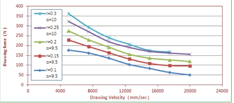
[image:8.595.113.498.490.730.2]Figure 8-b. Effect of drawing velocity on the drawing force at different of reduction in area .
5.2. Effect of Drawing Velocity on Drawing Force
In order to estimate the effect of velocity on the drawing force in the finite element software a node was selected on the wire surface at the die exit, see Figure (8-a), and the stress at this node was calculated.
One important parameter that affects the drawing force is the drawing velocity. The velocity is inversely proportional to the drawing force which means that any increase in velocity will cause a reduction in the drawing force at the same node, as shown in Figure (8-b). This figure shows the effect of drawing velocity (ν= 5000, 7500, 10000, 12500, 15000, 17500 and 20000) mm/sec on the drawing force, which was calculated using the optimum die angle at different deformation ratios ( r= 0.1, 0.15, 0.2, 0.25 and 0.3). It can be seen that the increase in the drawing velocity leads to considerable decrease in the value of the drawing force due to the increase in yield strength and the ultimate tensile strength for the material. These results agree with the results of Kabayama et al. [3] and Gawali et al.[5] .
Note that when r=0.3, Max. wire velocity is 17500 mm/sec as the wire drawing process fails if we have increased the velocity to a value more than 17500 mm/sec .
5.3. Statistical Analysis of Wire Drawing Results
The wire drawing results were treated statistically using the statistical packages of social sciences (SPSS) to achieve multi-variable analysis of variance to capture an equation which predicts the drawing force depending on the drawing parameters such as reduction in area (r), bearing length (BL) and semi-die angle (α). Also regression analysis was used to determine the effect of each parameter on drawing force. Additionally regression analysis was used to determine the effect of reduction in area (r) and semi-die angle (α) on the redundant factor.
5.3.1. Effect of Reduction in Area (r), Bearing Length (BL), Semi-Die Angle (α) on the Drawing Force (F)
The finite element results were analyzed with multi-variable analysis of variance to obtain an equation which predicts the drawing force under different drawing parameters (r, BL, α). Such an equation from this analysis can be written as:
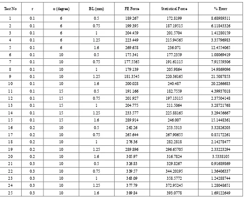
𝐷𝐷𝑟𝑟𝐷𝐷𝐷𝐷𝐷𝐷𝐷𝐷𝐷𝐷 𝐹𝐹𝐸𝐸𝑟𝑟𝐹𝐹𝐹𝐹 = 61.15 + 57.501 𝐵𝐵𝐵𝐵 + 1.104 𝛼𝛼 + 762.954 𝑟𝑟 (10) Table (5) explains the comparison between the finite element drawing force and the drawing force obtained from Equation (10), with the percentage error between the two values. The percentage error was calculated using the following equation.
𝐸𝐸𝑟𝑟𝑟𝑟𝐸𝐸𝑟𝑟 % = �𝐹𝐹𝐹𝐹𝐸𝐸− 𝐹𝐹𝑆𝑆𝐴𝐴𝑎𝑎𝐴𝐴𝐴𝐴𝑆𝑆.
𝐹𝐹𝐹𝐹𝐸𝐸 � × 100 % (11)
Where:
𝐹𝐹𝐹𝐹𝐹𝐹=Finite Element Drawing Force,
𝐹𝐹𝑆𝑆𝐴𝐴𝑎𝑎𝐴𝐴𝐴𝐴𝑆𝑆. = Statistical Drawing Force.
The average percentage error was calculated to be 5.79754248%. From Table (5) it can be noticed that the percentage error was small at small values of drawing condition and increased gradually with the increasing of the drawing condition values.
In order to calculate the correlation coefficient between the three drawing conditions (reduction in area, bearing length, semi-die angle) and its effects on drawing force, the finite element was treated using the regression analysis. First run involved the reduction in area only which gives a correlation coefficient of R=0.905 which means that reduction in area has a large effect on drawing force.
Table 5. Comparison between finite element drawing force and the calculated drawing force using equation (10). % Erorr Statistical Force FE Force BL (mm) α (degree) r Test No 8.68989311 172.8199 189.267 0.5 6 0.1 1 6.11843326 187.19515 199.395 0.75 6 0.1 2 1.41280159 201.5704 204.459 1 6 0.1 3 3.35796983 215.94565 223.449 1.25 6 0.1 4 12.4554065 236.071 269.658 1.6 6 0.1 5 1.08069419 177.2359 175.341 0.5 10 0.1 6 7.91559306 191.61115 177.5565 0.75 10 0.1 7 14.9869096 205.9864 179.139 1 10 0.1 8 21.5087853 220.36165 181.3545 1.25 10 0.1 9 20.2266683 240.487 200.028 1.6 10 0.1 10 4.39937018 182.7559 191.166 0.5 15 0.1 11 2.37504148 197.13115 201.927 0.75 15 0.1 12 3.28721768 211.5064 204.775 1 15 0.1 13 3.29456667 225.88165 233.577 1.25 15 0.1 14 15.1448361 246.007 289.914 1.6 15 0.1 15 3.32826203 253.5313 262.26 0.5 10 0.2 16 0.85172261 267.90655 265.644 0.75 10 0.2 17 2.14278477 282.2818 276.36 1 10 0.2 18 2.33223294 296.65705 289.896 1.25 10 0.2 19 3.5338105 316.7824 305.97 1.6 10 0.2 20 0.91689869 329.8267 326.83 0.5 10 0.3 21 1.36406337 344.20195 339.57 0.75 10 0.3 22 1.24288744 358.5772 363.09 1 10 0.3 23 1.28048651 372.95245 377.79 1.25 10 0.3 24 1.69122649 393.0778 399.84 1.6 10 0.3 25
Finally, the regression analysis was achieved using the reduction in area, bearing length, and semi-die angle. This analysis gives a correlation factor of R=0.963, note that the effect of semi-die angle on drawing force was also very small compared with reduction in area and less than the effect of bearing length as shown in Table (6).
[image:10.595.57.298.645.746.2]From the regression analysis it can be noticed that the reduction in area (r) has a large effect (90.5%) on the drawing force, bearing length (BL) has less effect of reduction in area (5.7%), and semi-die angle (α) has the less effect (0.1%) compared with reduction in area and bearing length.
Table 6. Regression analysis results.
Model R Square R Adjusted R Square Std. Error of the Estimate 1. reduction in area 0.905(a) 0.818 0.810 29.915232 2. reduction in area
+ bearing length 0.962(b) 0.925 0.918 19.615877 3. reduction in area
+ bearing length +
semi-die angle 0.963(c) 0.927 0.917 19.781521
5.3.2. Effect of Reduction in Area (r), Semi-Die Angle (α) on the Redundant Factor (ϕ)
The analytical results were analyzed with multi-variable analysis of variance to obtain an equation which predicts the redundant factor under different values of reduction in area (r) and semi-die angle (α). Such an equation from this analysis can be written as:
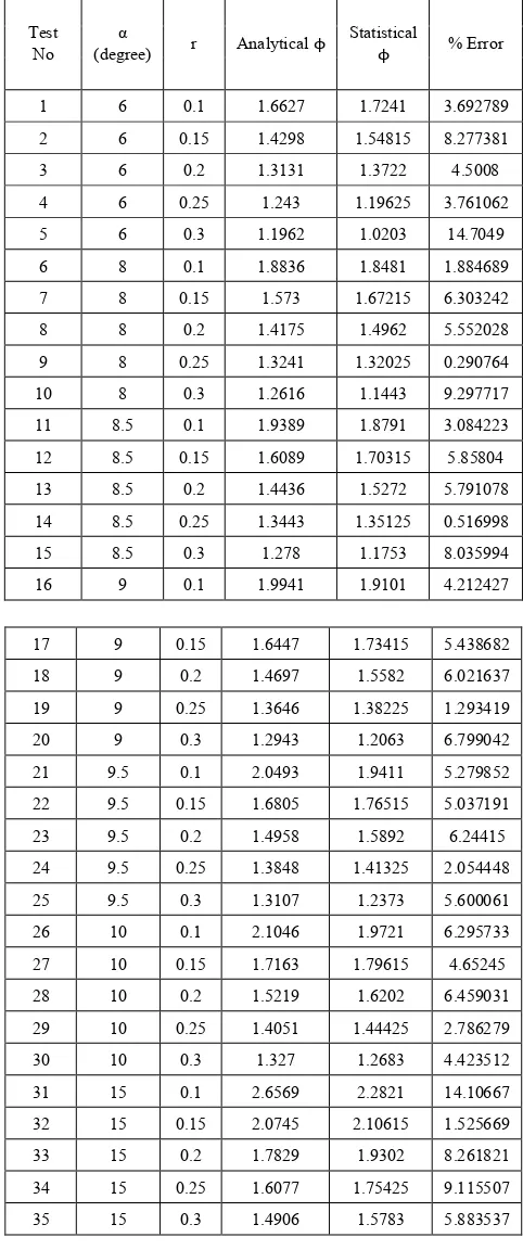
𝑅𝑅𝐹𝐹𝑅𝑅𝑅𝑅𝐷𝐷𝑅𝑅𝐷𝐷𝐷𝐷𝑅𝑅 𝐹𝐹𝐷𝐷𝐹𝐹𝑅𝑅𝐸𝐸𝑟𝑟 = 1.704 − 3.519 𝑟𝑟 + 0.062 𝛼𝛼 (12) Table (7) explains the comparison between the analytical redundant factor and the redundant factor obtained from Equation (12), with the percentage error between the two values. The percentage error was calculated using the following equation.
𝐸𝐸𝑟𝑟𝑟𝑟𝐸𝐸𝑟𝑟 % = �𝜑𝜑𝐴𝐴𝑛𝑛𝑎𝑎𝐴𝐴𝐴𝐴𝐴𝐴𝐴𝐴𝐴𝐴𝑎𝑎𝐴𝐴− 𝜑𝜑𝑆𝑆𝐴𝐴𝑎𝑎𝐴𝐴𝐴𝐴𝑆𝑆.
𝜑𝜑𝐴𝐴𝑛𝑛𝑎𝑎𝐴𝐴𝐴𝐴𝐴𝐴𝐴𝐴𝐴𝐴𝑎𝑎𝐴𝐴 � × 100 % (13)
Where:
𝜑𝜑𝐴𝐴𝑛𝑛𝑎𝑎𝐴𝐴𝐴𝐴𝐴𝐴𝐴𝐴𝐴𝐴𝑎𝑎𝐴𝐴=Analytical Redundant Factor,
𝜑𝜑𝑆𝑆𝐴𝐴𝑎𝑎𝐴𝐴𝐴𝐴𝑆𝑆. = Statistical Redundant Factor.
area and semi-die angle, and increased gradually with increasing the reduction in area and semi-die angle values.
Table 7. Comparison between analytical redundant factor and the redundant factor calculated using equation (12).
% Error Statistical
ϕ
Analytical ϕ
r α (degree) Test No 3.692789 1.7241 1.6627 0.1 6 1 8.277381 1.54815 1.4298 0.15 6 2 4.5008 1.3722 1.3131 0.2 6 3 3.761062 1.19625 1.243 0.25 6 4 14.7049 1.0203 1.1962 0.3 6 5 1.884689 1.8481 1.8836 0.1 8 6 6.303242 1.67215 1.573 0.15 8 7 5.552028 1.4962 1.4175 0.2 8 8 0.290764 1.32025 1.3241 0.25 8 9 9.297717 1.1443 1.2616 0.3 8 10 3.084223 1.8791 1.9389 0.1 8.5 11 5.85804 1.70315 1.6089 0.15 8.5 12 5.791078 1.5272 1.4436 0.2 8.5 13 0.516998 1.35125 1.3443 0.25 8.5 14 8.035994 1.1753 1.278 0.3 8.5 15 4.212427 1.9101 1.9941 0.1 9 16 5.438682 1.73415 1.6447 0.15 9 17 6.021637 1.5582 1.4697 0.2 9 18 1.293419 1.38225 1.3646 0.25 9 19 6.799042 1.2063 1.2943 0.3 9 20 5.279852 1.9411 2.0493 0.1 9.5 21 5.037191 1.76515 1.6805 0.15 9.5 22 6.24415 1.5892 1.4958 0.2 9.5 23 2.054448 1.41325 1.3848 0.25 9.5 24 5.600061 1.2373 1.3107 0.3 9.5 25 6.295733 1.9721 2.1046 0.1 10 26 4.65245 1.79615 1.7163 0.15 10 27 6.459031 1.6202 1.5219 0.2 10 28 2.786279 1.44425 1.4051 0.25 10 29 4.423512 1.2683 1.327 0.3 10 30 14.10667 2.2821 2.6569 0.1 15 31 1.525669 2.10615 2.0745 0.15 15 32 8.261821 1.9302 1.7829 0.2 15 33 9.115507 1.75425 1.6077 0.25 15 34 5.883537 1.5783 1.4906 0.3 15 35
In order to calculate the correlation coefficient between the (reduction in area, semi-die angle) and its effects on redundant factor, the analytical was treated using the regression analysis. First run involved the reduction in area
only which gives a correlation coefficient of R=0.792 which means that reduction in area has a large effect on redundant factor.
The second run involves both the reduction in area and semi-die angle which gives a correlation factor of R=0.939 and this leads to conclude that the effect of the semi-die angle is very small compared with the reduction in area as shown in Table (8).
[image:11.595.309.556.231.310.2]From the regression analysis it can be noticed that the reduction in area (r) has a large effect 79.2% on the redundant factor, and semi-die angle (α) has the less effect 14.7% compared with reduction in area.
Table 8. Regression analysis results.
Model R Square R R Square Adjusted Std. Error of the Estimate 1. reduction in area 0.792(a) 0.628 0.617 0.1972850 2. reduction in area
+ semi-die angle 0.939(b) 0.881 0.874 0.1132260
6. Conclusions
The following conclusions may be achieved from the results presented in this paper:
1. A DEFORM – 3D was successfully used to simulate the wire drawing process. The adopted model showed a reasonable agreement with the results of the analytical method with a maximum error of 4%.
2. For Aluminum -1100 the optimum die angle (9.5, 9.5, 9.5, 10˚ and 10˚) for each value of reduction in area (0.1, 0.15, 0.2, 0.25 and 0.3) respectively.
3. The increase of bearing length causes an increase in the drawing force, and to avoid the increase of drawing force, the reduction in area and friction coefficient should be small with a large die angle.
4. The drawing velocity has a significant effect on the drawing force, when the drawing velocity increases (at different reduction in area`) the drawing force decrease, for each material undergoes a certain range of velocities and failure taking place when the velocity goes out of this range.
5. The statistical results have shown that the most significant effect on the drawing force is the reduction in area, followed by the bearing length, and die angle although this was to a lesser degree during the drawing process of AL-1100.
REFERENCES
[1] E.M. Rubio, A.M. Camacho, L. Sevilla and M.A. Sebastián. Calculation of the forward tension in drawing processes, Journal of Materials Processing Technology, 162-163, pp. 551-557, 2005.
[3] L.K. Kabayama, S.P. Taguchi, G.A. Santana Martinez. The influence of die geometry on stress distribution by experimental and FEM simulation on electrolytic copper wiredrawing, Materials Research, Vol. 12, No. 3, pp. 281-285, 2009.
[4] G.Vega, A.Haddi , A.Imad. Investigation of process parameters effect on the copper-wire drawing, Materials and Design, 30, pp. 3308-3312, 2009.
[5] Prakash Gawali , Amitesh Paul , G. R. Selokar, " Effect of high speed drawing on properties of high carbon steel wires", International Journal of Modern Engineering Research, Vol.2, Issue.2, pp. 209-214, 2012.
[6] Cem S. Cetinarslan, " A Study on Influences of some Process Parameters on Cold Drawing of Ferrous Wires", Indian Journal of Engineering &Materials Sciences, Vol.19, pp. 221-228, 2012.
[7] Cem S. Cetinarslan , Ali Güzey, "Tensile properties of cold-drawn low-carbon steel wires under different process parameters", Professional Article, Issn 1580-2949, 2013. [8] George E. Dieter. Mechanical Metallurgy, McGraw-Hill
Book Company, (1961).
[9] Mikell P. Groover. Fundamentals of Modern Manufacturing: Materials, Processes, and Systems , 4𝐴𝐴ℎedition, John Wiley &
Sons, Inc, (2010).
[10] S. Kalpakjian and S. R. Schmid. Manufacturing Processes for Materials, 4𝐴𝐴ℎedition, Prentice Hall, (2003).
[11] Betzalel Avitzur. Metal Forming : processes and analysis, McGraw- Hill Book Company, (1968).
[12] George E. Dieter, Howard A. Kuhn and S. Lee Semiatin. Handbook of Workability and Process Design, ASM International, (2003).
[13] ASTM Designation : B 211 - 02. Stander Specification for Aluminum and Aluminum – Alloy Bar, Rod, and Wire . [14] ZDB Group. Drawing dies from sintered Carbides, Report
(Production catalogue), ZDB company Czech Republic. [15] Deform-3D V6.1 user manual, 2007,DesignEnvironment for
Forming.
[16] Robert B. Gifford . An investigation of product quality modification capabilities during wire drawing, M.Sc. Thesis, Lehigh University, Candidacy, Mechanical Eng. Department, 2000.
[17] H.I. Khalaf, Z.K. Radhi, S.M. Shrama. Temperature rise in Al 7075 cold wire drawing using finite element method, Thi-Qar University Journal for Engineering Sciences, Vol. 2, No. 2, 2011.
![Figure 1. A wide strip is being drawn through a frictionless die with a total included angle of 2α [8]](https://thumb-us.123doks.com/thumbv2/123dok_us/8758994.893548/2.595.313.552.155.272/figure-wide-strip-drawn-frictionless-total-included-angle.webp)