Exploding offers and buy now discounts

Munich Personal RePEc Archive

Exploding offers and buy-now discounts

Armstrong, Mark and Zhou, Jidong

University College London (UCL)

June 2011

Exploding O¤ers and Buy-Now Discounts

Mark Armstrong

University College London

Jidong Zhou

University College London

June 2011

Abstract

A common sales tactic is for a seller to encourage a potential customer to make her purchase decision quickly, before she can investigate rival deals in the market. We consider a market with sequential consumer search in which …rms can achieve this either by making an exploding o¤er (which permits no return once the consumer leaves) or by o¤ering a buy-now discount (which makes the price paid for immediate purchase lower than the regular price). We show that …rms often have an incentive to use these sales techniques, regardless of their ability to commit to their selling policy. We examine the impact of these sales techniques on market performance. Inducing consumers to buy quickly not only reduces the quality of the match between consumers and products, but may also raise market prices.

Keywords: Consumer search, oligopoly, price discrimination, high-pressure selling, exploding o¤ers, buy-now discounts, costly recall.

1

Introduction

Selling techniques are rarely a focus of economic research, although they are an important aspect of the consumer experience in many markets. One controversial sales method forces the consumer to decide quickly whether to buy. Methods of encouraging a quick decision include a seller refusing to sell to a customer unless she buys immediately (a sales tactic for which we use the term “exploding o¤er”), or the seller telling the potential customer that she will pay a higher price if she decides to purchase at a later date (we say the seller then o¤ers a “buy-now discount”). In his account of sales practices, Cialdini (2001, page 208) reports:

Customers are often told that unless they make an immediate decision to buy, they will have to purchase the item at a higher price later or they will be unable to purchase it at all. A prospective health-club member or automobile buyer might learn that the deal o¤ered by the salesperson is good for that one time only; should the customer leave the premises the deal is o¤. One large child-portrait photography company urges parents to buy as many poses and copies as they can a¤ord because “stocking limitations force us to burn the unsold pictures of your children within 24 hours”. A door-to-door magazine solicitor might say that salespeople are in the customer’s area for just a day; after that, they, and the customer’s chance to buy their magazine package, will be long gone. A home vacuum cleaner operation I in…ltrated instructed its sales trainees to claim that, “I have so many other people to see that I have the time to visit a family only once. It’s company policy that even if you decide later that you want this machine, I can’t come back and sell it to you.”

There are other examples of exploding o¤ers: an academic journal may o¤er to publish a paper if the author submits it immediately before trying her luck with another outlet, or a seller of life insurance may give a quote to a consumer which is valid only for 10 days, knowing that it will take the consumer more than 10 days to generate another quote given the medical tests required.

A less extreme sales tactic than banning return is to o¤er a discount for immediate sale. Bone (2006, pp. 71-73) documents how a home improvement company o¤ers its potential customers a regular price for the agreed service, together with a discounted price—which was termed a “…rst call discount”—if the customer agrees immediately. Robinson (1995) discusses other examples of buy-now discounts, such as a prospective tenant who is o¤ered an apartment for $900 per month but to whom the landlord o¤ers $850 if she agrees immediately, or a car dealer trying to close a deal who o¤ers a further $500 o¤ the price if the buyer accepts now, so (as he claims) he can then make his sales quota for that month. This paper examines a seller’s incentive to discriminate against customers who wish to buy later, after investigating rival o¤ers. It is natural to study this issue in the context of sequential search, where consumers search for a suitable product and/or for a low price.1

There are three leading models of sequential consumer search, each of which is relevant for

1_{We use a model with rational consumers. There are many other methods to induce sales which rely on}

the analysis in this paper. First, Diamond (1971) proposes a model in which sellers o¤er homogenous products, where consumers know their value for the product in advance of search, and where all consumers have a positive cost of searching for an additional price. In this situation, the “Diamond paradox” applies and the market can fail to operate at all: if consumers anticipate some equilibrium price P from sellers, then to search for a seller they must be willing to pay at leastP+sfor the product, which gives a seller an incentive to charge at leastP+s. Thus, there can be no equilibrium price which induces consumers to enter the market.

Second, Stahl (1989) modi…es Diamond’s model so that a fraction of consumers do not have search costs, and always investigate all options in the market. The presence of these “shoppers” gives …rms an incentive to set low prices, and the market is active. In equilibrium, …rms choose prices according to a mixed strategy, and there is price dispersion in the market. The shoppers buy the cheapest available product, while prices are low enough that those consumers with positive search costs buy from the …rst …rm they …nd. Third, Wolinsky (1986) proposes a model with product di¤erentiation, so that consumers need to search for a suitable product as well as a low price. Because consumers do not know their match utility from a …rm until they visit that …rm, the Diamond paradox need not arise even though all consumers have positive search costs. In equilibrium all …rms choose the same deterministic price, and consumers keep searching until they …nd a product with match utility above a threshold. (If no product’s utility is above the threshold, consumers go back to buy from the “least bad” option if that option yields a positive surplus.)

In the latter two search models, some consumers will return to buy from a previously sampled seller after investigating other sellers.2 _{In this paper we discuss how …rms may wish}

to discriminate against these return buyers. Of course, to do this a seller needs to be able to distinguish potential customers it meets for the …rst time from those who have returned after a previous visit. In the majority of circumstances this is not possible. (A supermarket, for instance, keeps no track of a consumer’s entry and exit from the store.) Nevertheless, in many markets such discrimination is feasible. A sales assistant may tell from a potential customer’s questions or demeanor whether she has paid a previous visit or not, or may simply recognize her face. In online markets, a retailer using tracking software may be able to tell if a visitor using the same computer has visited the site before. Sometimes—as with job o¤ers, automobile sales, tailored …nancial products, medical insurance, doorstep sales, or home improvements—a consumer needs to interact with a seller to discuss speci…c requirements, and this process reveals the consumer’s identity.

In such situations, there are two reasons why a …rm might wish to discriminate against those consumers who buy later. First, there is a strategic reason, which is to deter a

2_{De los Santos (2008) presents an empirical study of consumer search behaviour prior to making a}

potential consumer from going on to investigate rival o¤ers. If a consumer cannot return to a seller once she leaves, this increases the opportunity cost of onward search, as the consumer then has fewer options remaining relative to the situation in which return is costless. Second, the observation that a consumer has come back to a seller after sampling other options reveals relevant information about a consumer’s tastes or the prices she has been o¤ered elsewhere, and this may provide a pro…table basis for price discrimination. A seller may charge a higher price to those consumers who have already investigated other sellers, because their decision to return indicates they are unsatis…ed with rival products.3

As we will see, the former motive is most relevant when …rms can commit to their buy-later policies (or at least when some consumers believe that announced buy-later policies will be used), while the latter is more important when …rms have less commitment power.

A simple example may help …x some of the ideas used in this paper. A principal (a seller or an employer, say) makes an o¤er to a risk-neutral agent (a consumer or worker), knowing that the agent will receive another o¤er from a second principal subsequently. The …rst principal aims to maximize the probability that the agent accepts the o¤er. Suppose that the agent’s payo¤ from the …rst principal is u1 and her payo¤ from the second principal is

u2, where u1 and u2 are identical and independent random variables with mean u. When the agent receives her …rst o¤er, she (but not the …rst principal) observes u1 but does not yet know the realization of u2. Suppose the agent incurs no search or discounting costs to obtain the second o¤er, and always wishes to accept one o¤er or the other. If the …rst principal allows the agent to return freely after she receives her second o¤er, the agent will wait for the second o¤er and choose the better option, so that the agent accepts the …rst principal’s o¤er with probability equal to a half. However, if the …rst principal commits to an exploding o¤er so that the agent cannot come back if she waits for the second o¤er, then the agent accepts the exploding o¤er if u1 u. Thus, the exploding o¤er increases the probability of acceptance if and only if the mean of the distribution is below the median, so that the distribution is negatively skewed. The basic trade-o¤ involved is as follows. When the …rst principal uses an exploding o¤er, this makes the agent more likely to accept the o¤er immediately if she likes it, but it prevents the agent, in the event that she has only a moderate payo¤ from the o¤er, from coming back if she receives a worse o¤er from the second principal. When the distribution is negatively skewed, the …rst e¤ect dominates. Of course, the agent is harmed when the …rst principal makes an exploding o¤er, since she obtains her ideal outcome when free recall is allowed while an exploding o¤er leads to ine¢cient matching for some realizations of (u1; u2).

3_{This contrasts with the substantial literature on dynamic pricing, which examines how …rms can use}

In this paper we extend this illustrative example to allow for positive search costs and price competition between an arbitrary number of sellers, to allow sellers to set higher prices to return visitors (rather than merely to ban their return), to relax the assumption that sellers can commit to their buy-later policies, and to consider situations in which it is uncertainty about price rather than match utility which is relevant. For most of the paper we conduct the analysis in Wolinsky’s framework with product di¤erentiation, although at the end of the paper we verify that the main insight carries over to the alternative Stahl model with homogenous products and price dispersion. In section 2 we suppose that …rms can employ one of just two “buy-later” policies: consumers can freely return after leaving the …rm (and buy at the same price), or exploding o¤ers are used and …rst-time visitors are forced to buy immediately or never. We show that …rms wish to use exploding o¤ers when the consumer demand curve is concave (which is akin to the negative skewness needed in the simple example above), while when demand is convex …rms choose to allow free recall. Beyond cases of convex or concave demand, we show that exploding o¤ers are typically an equilibrium sales technique when search frictions are large and there are many suppliers. We derive the equilibrium price when all …rms use exploding o¤ers, and …nd that this price can be higher or lower than the corresponding price with free recall.

In section 3 we assume …rms have a richer set of buy-later policies from which to choose, and rather than simply banning return they can charge their returning visitors a higher price. We …rst analyze the case where …rms can commit to their buy-later price. Starting from a situation in which …rms treat …rst-time and returning consumers symmetrically, we show under mild conditions that a …rm has an incentive to o¤er a buy-now discount. We derive the equilibrium prices for immediate and returning purchase in a duopoly example, and because of the extra search frictions introduced by the buy-now discount, even the discounted buy-now price can be higher than the non-discriminatory price.

is identical to the full commitment outcome.

In section 4 we discuss alternative reasons why …rms may wish to encourage quick decision making. We examine a model with homogenous products and price dispersion as in Stahl’s search model. Here, a consumer’s uncertainty about future options concerns price rather than match utility. The results are more clear-cut relative to the setting where products are di¤erentiated, and starting from Stahl’s free-recall equilibrium we show that a …rm always has a unilateral incentive to make an exploding o¤er. We also discuss how consumer risk aversion makes it more likely that exploding o¤ers are a pro…table strategy, how an incumbent …rm can employ exploding o¤ers so as to deter a more e¢cient entrant, and why a …rm may force a quick decision in order to prevent consumers from comprehending the current product (as opposed to the products o¤ered by rival sellers).

As far as we know, this paper is the …rst to study the use of exploding o¤ers (or, more generally, buy-now discounts) in consumer markets. In the alternative setting of matching markets, however, there are a number of studies in which exploding o¤ers play a role. Exploding o¤ers are often used in specialized labor markets, such as those for law clerks, sport players, medical sta¤, and student college allocations. In such markets, …rms make o¤ers to which applicants must respond quickly, and these markets often clear very fast, with …rms as well as applicants having little opportunity to consider their alternatives. (See Roth and Xing, 1994, for an account of a number of such markets.) This literature often studies exploding o¤ers, together with early contracting, in a setting where match quality information (e.g., information about workers’ productivity) is revealed over time (see Li and Rosen, 1998, for instance). When exploding o¤ers are used, these markets have a tendency to “unravel”: employers compete to make and workers are willing to accept ever earlier o¤ers. Early contracting can provide an insurance gain for agents, but it causes ine¢cient matching. Niederle and Roth (2009) conducted an experimental study on the use of exploding o¤ers in a laboratory matching market. They …nd that …rms do tend to use exploding o¤ers when they are permitted to do so, and the result is that matching occurs ine¢ciently early and match quality is poor, relative to the situation in which using exploding o¤ers is banned. Our model is more suitable for consumer markets where the interaction between buyers and sellers often occurs through individual search processes instead of through a synchronized matching market as often seen in labor markets. But both early contracting in labor markets and early buying in our model lead to an ine¢cient use of information available in the market.

further show that equilibrium prices do not depend on the recall cost.4

Firms often bene…t from a reduction in consumer search intensity, since this usually softens price competition. In our model, the exploding o¤er or buy-now discount serves this purpose. Alternatively, Ellison and Wolitzky (2008) extend Stahl’s model so that a consumer’s incremental search cost increases with her cumulative search e¤ort. If a …rm increases its in-store search cost (say, by making its tari¤ harder to comprehend), this will make further search less attractive. They show that if the exogenous component of search costs falls, …rms will unilaterally increase their self-determined element of search costs, with the result that equilibrium prices are unchanged. Though otherwise very di¤erent, our model and theirs study how search frictions are determined endogenously: even if intrinsic search frictions are negligible, a market may su¤er from substantial search frictions—and high prices—in equilibrium.

Finally, our analysis of buy-now discounts is related to the literature on auctions with a “buy now” price (see Reynolds and Wooders, 2009, for instance). Online auctions some-times o¤er bidders the option to buy the item immediately at a speci…ed price rather than enter an auction against other bidders. In these situations, a seller has one item to sell to a number of potential bidders, and so a bidder needs to pay a high buy-now price in order to induce the seller from going on to search for other bidders by running an auction, whereas our model involves sellers o¤ering alow buy-now price so as to induce a buyer from going on to search for other sellers. Common rationales for buy-now prices in auctions are impatience or risk-aversion on the part of bidders or the seller, neither of which is needed in our model.

2

Exploding O¤ers

Our underlying market is based on Wolinsky’s model with di¤erentiated products.5 _There

are 2 n < ₁ symmetric …rms in the market, each supplying a single horizontally di¤erentiated product at a constant marginal cost which is normalized to zero.6 _{There are}

a large number of consumers with idiosyncratic preferences, and their measure is normalized to one. A consumer’s valuation of product i, ui, is a random draw from some common

4_{Daughety and Reinganum (1992) make the point that the extent of consumer recall may be}

endoge-nously determined by …rms’ equilibrium strategies. In their model, the instrument that a …rm can use to in‡uence consumer recall is the length of time that it will hold the good for consumers at the quoted price. In contrast to our assumption that a consumer can discover a seller’s buy-later policy only after investigating that seller, Daughety and Reinganum suppose that sellers can announce their recall policies to the population of consumers before search begins.

5_{See Anderson and Renault (1999) for analysis of a variant of Wolinsky (1986) in which there is no}

outside option and consumers always buy a product in the market.

6_{Note that if there were unlimited …rms in the market (n=1), banning or discouraging return has}

distribution with support [0; umax] and with cumulative distribution function F( ) and continuously-di¤erentiable and bounded density f( ). We suppose that the realization of match utility is independent across consumers and products. In particular, there are no systematic quality di¤erences across the products. Each consumer wishes to buy one item, provided an item can be found with a positive surplus. We sometimes refer to the function

1 F( )as the consumer demand curve.

Consumers initially have imperfect information about the deals available in the market. They gather this information through a sequential search process, and by incurring a search cost s 0, a consumer can visit a …rm and …nd out (i) its price, (ii) its “buy-later” policy, and (iii) the realized match value. (If the search cost is zero, we require that consumers nevertheless consider products sequentially.) In this section, the only two buy-later policies available to a …rm are to use an exploding o¤er or to allow free recall. (If a …rm allows free recall, it sets the same price to …rst-time visitors and returning visitors.) To implement an exploding o¤er, …rms are assumed to be able to distinguish …rst-time visitors from returning customers and to have the ability to commit not to serve a returning customer. After visiting one …rm, a consumer can choose to buy at this …rm immediately or to investigate another …rm. If permitted, she can costlessly return to a previous …rm after sampling subsequent …rms.7 _{Since …rms areex ante symmetric, we consider situations with random}

search, so that a consumer is equally likely to investigate any of the remaining unsampled …rms when she searches, and we also focus on symmetric equilibria.

The timing of the game is as follows. At the …rst stage, …rms set prices and buy-later policies simultaneously. The strategy space of each …rm is thenR+ ffree recall, exploding o¤er_g. At the second stage, consumers search sequentially and make their purchase decision after search is terminated. Consumers do not observe …rms’ actual choices before they start searching, but hold rational expectations of equilibrium prices and buy-later policies. Information unfolds as the search process goes on, but consumers’ beliefs about the o¤ers made by unsampled …rms are unchanged, even if they observe o¤-equilibrium o¤ers from some …rms. Both consumers and …rms are assumed to be risk neutral. We use the concept of perfect Bayesian equilibrium, and focus on symmetric pure strategy equilibria in which …rms set the same price and buy-later policy based on their expectation of consumers’ search behavior, and at each …rm consumers hold equilibrium beliefs about unsampled …rms’ strategies and make their search decisions accordingly.

A piece of notation which summarizes the distribution of match utilities and the extent of search frictions is

V(p)

Z umax

p

(u p)dF (u) s : (1)

7_{In most search markets, even if …rms allow free return, consumers face some intrinsic cost of returning}

Thus, V(p) is the expected surplus of sampling a product if a consumer expects that the price will bep, the cost of sampling the product iss, and this is the only product available. Note that V(p) is decreasing but p+V(p) is increasing in p. Throughout this paper we assume that the search costs is relatively small, so that

V(pM)>0; (2)

where pM is the monopoly price which maximizes p[1 F(p)]. This condition means that consumers are willing to sample a product sold even at the monopoly price. In the example where u is uniformly distributed on [0;1], which we use for illustration in the following analysis, condition (2) requiress < 1

8.

In the remainder of section 2, we compare market performance when …rms allow free recall with the situation where …rms make exploding o¤ers (sections 2.1 and 2.3), and we discuss the incentive …rms have to make exploding o¤ers (section 2.2).

2.1

The market with free recall and with exploding o¤ers

Here, we examine the market when all …rms allow free recall and compare this to the less familiar situation where all …rms make exploding o¤ers. If all …rms allow free recall, the situation is as in Wolinsky (1986), and for reference later we recapitulate part of his analysis. In a symmetric equilibrium in which all …rms set the same price p0, consumers have a stationary stopping rule whereby they buy a product immediately if they obtain a match utility u greater than a threshold a, and if no product yields that level of utility, the consumer samples all products and buys from the best of then options provided that option generates a positive surplus. Here, the reservation utility a is determined by the formula

V(a) = 0 : (3)

The expression Rumax

a (u a)dF (u) in V(a) is the incremental bene…t of searching once more if the best current utility is a and the consumer has free recall. So the optimal threshold makes the consumer indi¤erent between searching on, which incurs cost s, and purchasing this product with utilitya. SinceV( )is a decreasing function, (3) has a unique solution and a decreases with s, and condition (2) is equivalent to a > pM. Note that in this case there is e¢cient matching of consumers to products in the sense that a consumer will always buy her most preferred product from those products she sees.

The following result describes the equilibrium price in the market with free recall.8

Lemma 1 In the market where all …rms allow free recall, the …rst-order condition for p0

to be the equilibrium price is

1 F (p0)n

p0

+n

Z a

p0

F(u)n 1f0

(u)du =f(a)1 F(a) n

1 F(a) : (4)

8_{The …rst-order condition (4) was derived in Wolinsky (1986), while the results about existence and}

If the demand curve 1 F is strictly logconcave, then in the interval 0 < p0 < a the

…rst-order condition (4) has a solution and any such solution lies in the range

1 F(a)

f(a) < p0 < pM :

If the monopoly pro…t function p[1 F(p)]is concave, then the …rst-order condition (4) is su¢cient for p0 to be the equilibrium price.

(Unless otherwise stated, all omitted proofs can be found in the appendix.)

As the number of suppliers becomes large, the equilibrium price in (4) converges to

p0 = 1_fF_(a)(a). As the search cost tends to its upper bound in (2) (i.e., as a tends to pM), consumers stop searching whenever they …nd a product with positive surplus and each …rm acts as a monopolist, so the price converges top0 =pM (which then also equals 1_fF_(a)(a)).

Suppose next that all …rms force their …rst-time visitors to buy immediately or not at all. Suppose consumers anticipate that each …rm sets the price p. What is a consumer’s optimal search strategy? As is intuitive, consumers become less choosy as they run out of options, and their reservation utility for purchasing decreases the fewer …rms remain to be searched. Indeed, if they are unfortunate enough to reach the …nal …rm they will have to accept any o¤er which leaves them non-negative surplus. In particular, since a consumer may end up buying a product which is inferior to products rejected earlier in her search process, the matching of products to consumers is less e¢cient than in the market with free recall. The precise stopping rule is derived in the following result.9

Lemma 2 Suppose consumers face a search market with m …rms, each of which makes an exploding o¤er and sets price p. Then a consumer will enter the market if and only if

p < a, where a is given in (3), in which case she obtains expected surplus

Wm am p 0 ;

where am solves the recursive equation

am+1 =am+V(am) (5)

with initial value a0 =p and where V( ) is de…ned in (1). If p < a, a consumer who has

l 0 …rms remaining unsampled will buy from her current …rm if match utility is greater than al, and the sequence a0; a1; ::: is increasing.

Note that, unlike the case with free recall, each am depends on the price p since the starting value a0 does so. Note also that whenp < a the sequenceam in (5) converges to the free-recall reservation utility a asm _{! 1}.

9_{Related analysis of the optimal stopping rule for search without recall has been derived by, for example,}

We next derive the symmetric equilibrium price when …rms use exploding o¤ers. Sup-posen 1…rms set the pricepand the remaining …rm is considering its choice of price, say

~

p. (Of course, when choosing their search strategy consumers anticipate that this …rm has set the equilibrium price p.) Suppose this deviating …rm happens to be in the kth position

of a consumer’s search process, so n k …rms remain unsampled. Then the probability that the consumer will visit this …rm is h1 1 if k = 1, and if k >1 this probability is

hk k 1

Y

i=1

F(an i): (6)

From Lemma 2, she will then buy from this …rm if u p > a~ n k p, which occurs with probability1 F(an k p+ ~p), and so the …rm’s demand given it is in the consumer’s kth

search position is

hk[1 F(an k p+ ~p)]: (7) Since the …rm is in any position 1 k n with equal probability, its total demand with price p~when all other …rms are expected to set pricepis

Q(~p) = 1

n

n

X

k=1

hk[1 F(an k p+ ~p)];

and its pro…t is pQ~ (~p). The following result characterizes the equilibrium price when exploding o¤ers are used.10

Lemma 3 In the market where all …rms make exploding o¤ers, the …rst-order condition for p to be the equilibrium price is

p=

Pn

k=1hk[1 F(an k)]

Pn

k=1hkf(an k)

: (8)

If the demand curve 1 F is strictly logconcave, then in the relevant interval 0 < p < a

the …rst-order condition (8) has a solution and any such solution lies in the range

1 F(a)

f(a) < p < pM :

If the monopoly pro…t function p[1 F(p)] is concave, the …rst-order condition (8) is su¢cient for p to be the equilibrium price.

Since each an k depends on p, equation (8) de…nes p only implicitly. Notice that the numerator in the right-hand side of (8) equals 1 Qn_k=1F(an k), the total output in equilibrium.

10_{Lemmas 1 and 3 do not discuss the uniqueness of equilibria in the respective regimes. However, one can}

One can show that as the number of …rms tends to in…nity, this equilibrium price converges to the same lower bound 1_f(a)F(a) as in the free-recall case. Intuitively, when the number of …rms is unlimited, a consumer would never choose to return to a previously sampled …rm, even if she could freely do so, and so the use of exploding o¤ers has no e¤ect on the equilibrium price. Finally, as the search cost tends to its upper bound (i.e., as a

tends topM), p converges to the monopoly price pM as in the free-recall regime.

2.2

Incentives to make an exploding o¤er

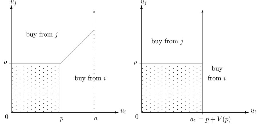
Before we compare the outcome when all …rms use exploding o¤ers with the benchmark model with free recall, we …rst investigate a more fundamental issue: when will …rms use exploding o¤ers in equilibrium? That is, if all its rivals make exploding o¤ers and set the price pin (8), does a …rm have an incentive to deviate and allow free recall (and, possibly, set a di¤erent price as well)? Before pursuing the analysis in general, consider this simple duopoly example with …xed prices which yields the main insight.

-6 a p p p p p p p p p p p p p p p p p p p p p p 6 0 _p p ui uj

buy fromi

buy fromj

p p p p p p p p p p p p p p p p p p p p p p p p p p p p p p p p p p p p p p p p p p p p p p p p p p p p p p p p p p p p p p p p p p p p p p p p p p p p p p p p p p p p p p p p p p p p p p p p p p p p p p p p p p p p p p p p p p p p p p p p p p p p p p p p p p p p p p p p p p p p p p p p p p p p p p p p p p p p -6 6 0 _a

1 =p+V(p)

p

ui

uj

buy fromi

buy fromj

p p p p p p p p p p p p p p p p p p p p p p p p p p p p p p p p p p p p p p p p p p p p p p p p p p p p p p p p p p p p p p p p p p p p p p p p p p p p p p p p p p p p p p p p p p p p p p p p p p p p p p p p p p p p p p p p p p p p p p p p p p p p p p p p p p p p p p p p p p p p p p p p p p p p p p p p p p p p p p p p p p p p p p p p p p p p p p p p p p p p p p p p p p p p p p p p

Figure 1a: Demand with free recall Figure 1b: Demand with exploding o¤er

implies that a consumer will buy from it if and only if ui > a1 = p+V(p). This pattern of demand is depicted in Figure 1b.

As we have shown, a1 2(p; a) and so the use of an exploding o¤er makes a consumer more likely to buy immediately, but it eliminates the possibility that the consumer comes back after …nding an inferior product elsewhere. One can calculate that whenuis uniformly distributed on[0;1], …rmi’s demand in the two …gures is identical, and when a …rm forces immediate sale this has no net impact on its demand. More generally, as in the illustrative example discussed in the introduction, the impact of using an exploding o¤er is to eliminate the …rm’s demand from “low ui” consumers, who have match utility close to price p and might otherwise come back, and to boost its demand from “high ui” consumers, who do not wish to risk losing the existing desirable option by going on to sample the rival. If

u has an increasing density (i.e., the demand curve 1 F is concave), the latter e¤ect dominates the former, and the net impact of forcing immediate sale is to boost a …rm’s demand. Similarly, if the demand curve is convex, then the former e¤ect dominates and the probability of a consumer accepting its o¤er is reduced when an exploding o¤er is used. The next result shows that this argument is valid with any number of …rms and en-dogenous prices.

Proposition 1 (i) If the demand curve 1 F is strictly concave then every symmetric equilibrium involves …rms using exploding o¤ers;

(ii) if the demand curve 1 F is strictly convex then every symmetric equilibrium involves …rms allowing free recall;

(iii) if the demand curve1 F is linear, i.e., uis uniformly distributed, then an equilibrium with exploding o¤ers and an equilibrium with free recall both exist.

This result only covers situations with concave or convex demand (i.e., where the density for the match utility is monotonic). The reason why results are then clear-cut is that the impact of exploding o¤ers on a …rm’s demand does not depend on the prevailing price. With a non-monotonic density function, whether exploding o¤ers are an equilibrium sales technique may depend on price. In particular, it may depend on both the number of …rms in the market and the magnitude of search frictions. Results with non-monotonic densities can be obtained if there are many suppliers, as described in the next result.11

Proposition 2 Suppose f is a hump-shaped density with mode u (i.e., f is strictly in-creasing for u < u and strictly decreasing for u > u ). Then for su¢ciently large n: (i) if a < u it is an equilibrium for all …rms to use exploding o¤ers;

(ii) if a > u it is an equilibrium for all …rms to allow free recall.

11_{From the proof of this result, one can also see that ifa < u , then for largenfree recall cannot emerge}

Loosely speaking, when n is large only the behavior of f around the threshold pointa

matters for the incentives to make an exploding o¤er. (Proposition 1 by contrast showed that exploding o¤ers are used when the density is everywhere increasing.) This result implies that when the density is hump-shaped and the number of …rms is large, the size of search frictions determines the equilibrium sales policy. When the search cost is high enough that a is smaller than the mode, …rms use exploding o¤ers; otherwise, …rms allow free recall. In particular, in “competitive” markets (in the sense that search frictions are small and the number of suppliers is large), we anticipate that allowing free recall is an equilibrium policy. The other useful comparative statics exercise is to consider the impact of the number of …rms on the equilibrium sales policy. To illustrate this in an example, consider the case where match utilities follow the hump-shaped Weibull distribution with

F (u) = 1 e u3

and support [0;₁), which has mode u 0:87 and monopoly price

pM 0:69. For a search cost such that a = 1> u , one can verify that when n= 2;3and 4the only symmetric equilibrium involves …rms using exploding o¤ers, while forn = 5and

6 all …rms allow free return.12

Our analysis presumed that consumers search through market options in a purely ran-dom order. In some markets, however, a prominent seller may attract a disproportionate share of initial consumer searches. (De los Santos (2008) showed this was so in the online book market.) Indeed, the examples of doorstep selling mentioned in the introduction do not …t the random search assumption well since such a seller is relatively likely to be the …rst seller for that product encountered by the consumer over the relevant time horizon. Nevertheless, prominence does not a¤ect a …rm’s incentive to adopt exploding o¤ers, at least when the demand curve is concave or convex, and Proposition 1 applies regardless of the fraction of …rst-time visitors a given seller receives. The reason can be understood by looking at Figure 1. The decision about whether or not to use an exploding o¤er only a¤ects a …rm’s demand from those consumers who sample it …rst, and this demand e¤ect is positive (negative) if the demand curve is concave (convex), independent of the proportion of such consumers. Thus, much of the analysis in this paper applies equally to situations where some sellers are more prominent than others.

Our analysis to this point relies on a …rm’s ability to commit to an exploding o¤er. However, if a consumer does come back to a …rm after sampling a rival, the …rm will have an incentive to sell to that consumer.13 _{This credibility problem is enhanced by the fact}

12_{See our online appendix for the details of these calculations. A second factor which could arise with}

non-monotonic densities is that …rms may choose intermediate buy-later policies, which make return costly for their …rst-time visitors but not prohibitively so. For example, online sellers can ask customers to log on to their accounts or input information again, or …rms can ask consumers to queue again or make another appointment if they want to come back. With a monotonic density, a …rm wishes either to make return impossible or free, even if it could impose intermediate returning costs.

13_{Indeed, the quote from Cialdini in the introduction immediately goes on to say: “This, of course, is}

that consumers oftenwill wish to return to previous …rms, since their stopping rule is such that their remaining option may have lower utility than previously rejected options. Even if …rms lack any ability to commit, though, …rms may wish to claim to employ exploding o¤ers if a fraction of consumers are “credulous”. When some consumers mistakenly believe a seller’s claim that they must buy immediately or not at all, then Proposition 1 still applies. To see this, notice that the other, rational, consumers will ignore what the sellers say about their buy-later policies and behave as in the free-recall case. So the decision about whether to make an exploding o¤er depends only on the credulous consumers who behave just as the consumers do in the full commitment case.14 _{In addition, as we discuss}

in section 3.3, when the more ‡exible sales policy with buy-now discounts is available, the lack of commitment power can strengthen a …rm’s incentive to discriminate against consumers who buy later.

2.3

The impact of exploding o¤ers

It is hard in general to compare market performance with and without the use of exploding o¤ers, and the comparison between the prices in (4) and (8) is opaque. To gain further insights consider …rst the case of a uniform distribution for match utility, so that u is uniformly distributed on [0;1] and the demand curve is linear. In this example, the …rst-order condition for the free-recall equilibrium price in (4) simpli…es to

1

p0

=pn₀ 1+ 1 a n

1 a ; (9)

while (8) implies that the equilibrium price with exploding o¤ers satis…es

1

p =hn+

n

X

k=1

hk (10)

wherehk=

Qk 1

i=1 an i is the probability in the exploding-o¤er equilibrium that a consumer will visit the kth …rm in her search order.15 (Lemmas 1 and 3 imply that these …rst-order

conditions are su¢cient forp0andpto be the equilibrium price in each regime.) Expression (5) implies that the reservation utility thresholds in the exploding o¤er regime satisfy

am+1 = 1 2(a

2

m+ 1) s

starting with a0 = p. As m becomes large am converges to a = 1

p

2s, the free-recall threshold. (Recall that in this uniform example condition (2) requiress < 1

8, i.e., a > 1 2.)

14_{While the proportion of credulous consumers does not a¤ect the incentive to use exploding o¤ers (at}

least when the demand curve is convex or concave), this proportion will a¤ect the equilibrium price when exploding o¤ers are (claimed to be) used. A conceptual issue arising in such a model with both rational and naive consumers is how they form their expectation of equilibrium prices. Our discussion here implicitly assumes that all consumers somehow hold the correct expectation about prices.

The following result shows that the price rises when exploding o¤ers are used in this example.

Proposition 3 Suppose u is uniformly distributed on [0;1] and s < 1

8. Then price is

higher when …rms use exploding o¤ers than when they allow free recall.

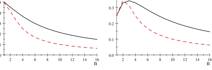
The solid curve in Figure 2a depicts how the exploding-o¤er price p varies with the number of …rms for the case s = 0, while the dashed curve depicts the free-recall price

p0. Both prices converge to zero for large n, but it seems that prices with exploding o¤ers are approximately double those which prevail with free recall. (This …gure includes the monopoly casen = 1, in which case the monopolist charges the price pM = 1₂ and the use of exploding o¤ers has no impact.) As the search cost gets larger, the di¤erence between the exploding-o¤er and free-recall prices decreases (and ifs = 1₈, the di¤erence vanishes).

2 4 6 8 10 12 14 16

0.0 0.1 0.2 0.3 0.4 0.5

n 2 4 6 8 10 12 14 16 0.0

0.1 0.2 0.3

n

Figure 2a: Prices with exploding o¤ers Figure 2b: Pro…ts with exploding o¤ers

In general, though, it is possible that prices remain unchanged or even fall when ex-ploding o¤ers are used, as the following examples demonstrate.16

Consider the exponential distribution with a c.d.f. F(u) = 1 e u= _{de…ned on} [0;₁), where is the expected value of match utility. Then one can verify that

p=p0 = , i.e., the use of exploding o¤ers has no impact on equilibrium prices.17

16_{In the …rst two of the following examples, although the demand curve is well-behaved in the sense}

that1 F is logconcave, the monopoly pro…t functionp[1 F(p)]is not concave as required by Lemmas 1 and 3. But one can numerically verify that a …rm’s pro…t function is nevertheless single-peaked, so that …rst-order condition is su¢cient forp0andpto be the equilibrium prices.

17_{The special feature of the exponential distribution is that a monopoly …rm facing this population of}

consumers, where each consumer has an outside option with utility z 0, will choose the same price

Consider the Weibull distribution with a c.d.f. F(u) = 1 e u2

de…ned on [0;₁), where the monopoly price is pM 0:71. Whenn = 2 and a= 10, one can show that

p 0:63< p0 0:64.

Finally, consider the distribution with density functionf(u) = 1₂+_1+e k1(u 1=2) de…ned

on[0;1](which is a truncated logistic function). For k >0, this density is increasing and so the demand curve1 F is concave. Whenk = 50(in which case the monopoly price ispM 0:53),n = 2 and a= 0:6, one …nds that p 0:4997< p0 0:5054.

Therefore, the comparison of prices in the free-recall and the exploding-o¤er regimes is ambiguous, even with reasonable regularity conditions placed on the demand function. The reason why it is hard to obtain clear-cut results about the impact of exploding o¤ers on price is that there are a number of distinct e¤ects at work. On one hand, using exploding o¤ers makes …rst-time visitors less likely to search on, which tends to reduce a …rm’s demand elasticity since fewer consumers can compare prices across …rms. On the other hand, using exploding o¤ers excludes potential returning consumers, the demand from whom is typically rather inelastic, and which therefore may raise demand elasticity.18 _On

top of these two potentially con‡icting e¤ects, for a given price the use of exploding o¤ers excludes more consumers from the market, which also a¤ects the demand elasticity. As a result, the net impact of the use of exploding o¤ers on price depends on the shape of the demand curve in a complex way.

Whenever p p0 (such as in the uniform or exponential examples), aggregate con-sumer surplus and total welfare (measured by the sum of concon-sumer surplus and pro…t) fall when all …rms use exploding o¤ers, relative to the situation when all …rms allow free recall. Consumer surplus falls since the price rises compared to the free-recall situation

and consumers are prevented from returning to a product which yields positive surplus. (Even if p=p0, i.e., if using exploding o¤ers did not change the market price, consumers would obtain lower surplus in the exploding-o¤er case due to the no-return restriction. The higher pricep > p0 only adds to their loss.) As far as total welfare is concerned, relative to the free-recall situation, the use of exploding o¤ers not only induces suboptimal matching (i.e., consumers on average cease their search too early due to the “buy now or never” requirement), but also excludes more consumers from the market since p p0, both of which harm e¢ciency.

However, it is ambiguous whether the exploding-o¤er equilibrium has a higher pro…t level than the free-recall equilibrium even if p > p0. Figure 2b above compares industry pro…t between the two cases in the uniform example withs= 0 (the solid curve represents the exploding-o¤er case). The pro…t is lower with exploding o¤ers when n = 2. For a

18_{To understand the elasticity of the returning customers, consider the …nal integral term in (19) in the}

higher search cost, this can happen with a greater number of …rms (e.g., when s = 0:05, it is true for n 4). In the above logistic example, one can also check that …rms earn less in the exploding-o¤er equilibrium than in the free-recall equilibrium. Together with Proposition 1, these examples indicate that …rms may end up playing a prisoner’s dilemma when they are able to use exploding o¤ers: each …rm has a unilateral incentive to use an exploding o¤er, but when all …rms do so their pro…ts fall.

3

Buy-Now Discounts

An alternative framework allows a …rm to charge a higher price to returning visitors instead of the drastic measure of banning return. When this more ‡exible sales policy is available, we will show that a …rm’s incentive to discriminate against returning customers is present under more general conditions than needed for Proposition 1. Consider the same model as before, except that instead of choosing the extreme policies of either allowing free return or no return, each …rm can choose two distinct prices: p is the price for …rst-time visitors and p^is the price for returning customers, and the strategy space of each …rm becomes

R+ R+. (Neither price is observable to consumers before they start searching.) Whenever

^

p > p, returning to a previous …rm is costly.19 _{Indeed, whenp^is su¢ciently high, the …rm}

in e¤ect makes an exploding o¤er. One interpretation of this discriminatory pricing is that a …rm sets a regular (or “buy-later”) price p^ and o¤ers …rst-time visitors a “buy-now” discount p^ p. Until section 3.3, we assume that a …rm can commit top^when it o¤ers new visitors the buy-now price p.

3.1

Incentives to o¤er a buy-now discount

We …rst analyze when a …rm has an incentive to o¤er a buy-now discount , starting from the situation in which all …rms o¤er the equilibrium uniform price p0 in expression (4). First, we observe that the impact of o¤ering a small buy-now discount on a …rm’s pro…t is just as if the …rm levies a small buy-later premium.20

19_{Ifp < p^ , then a consumer has an incentive to leave a …rm and then return, even if she has no intention}

of investigating other …rms. If this kind of consumer arbitrage behavior—of stepping out the door and then back in again—cannot be prevented, then settingp < p^ is equivalent to setting a uniform price p^, and so without loss of generality we assume …rms are constrained to setp^ p.

20_{Suppose all …rms but one choose the uniform pricep}

0in (4). If the remaining …rm o¤ers the buy-now

pricepand buy-later pricep+ , denote this …rm’s pro…t by (p; ). Ifp p0 and 0, then

(p; ) (p0;0) + (p p0) p(p0;0) + (p0;0) = (p0;0) + (p0;0);

where the equality follows from the assumption that p0 is the equilibrium uniform price and subscripts

denote partial derivatives. Thus, the impact on the …rm’s pro…t is captured by the term (p0;0), which

Lemma 4 Starting from the situation in which all …rms o¤er the equilibrium uniform price p0 in (4), the impact on a …rm’s pro…t of o¤ering a small buy-now discount (so its

buy-now price is p0 and its buy-later price isp0) is approximately equal to the impact of

levying a buy-later premium (so its buy-now price is p0 and its buy-later price is p0+ ). Intuitively, the fact that p0 is the equilibrium uniform price implies that a …rm’s pro…t is not signi…cantly a¤ected by small changes in its uniform price, and the only …rst-order impact on a …rm’s pro…t comes from its buy-now discount (regardless of whether this is interpreted as a discount for immediate purchase relative to the buy-later price p0, or as a premium for later purchase relative to the buy-now price p0).

To illustrate the pros and cons of o¤ering a discount most transparently, consider initially the case of duopoly. It is somewhat more straightforward to consider the incentive to charge a buy-later premium, and then to invoke Lemma 4. If …rm i introduces a buy-later premium, this has no impact on its demand and pro…t from those consumers who …rst sample the rival given they hold equilibrium beliefs, and so we can restrict attention to that portion of consumers who sample …rm i …rst. A buy-later premium not only discourages consumers from searching on, as the exploding o¤er did in the earlier analysis, but also generates extra revenue from returning consumers.

How does a¤ect a consumer’s decision whether to buy immediately from …rm i? Denote by a( ) the reservation utility which leads the consumer to buy immediately, i.e., if she …nds match utilityui a( ) at the …rm she will buy without investigating the rival. Clearly if no premium is levied ( = 0) then a(0) = a, the free-recall reservation level in (3). By de…nition, if a consumer discovers utility ui = a( ) at …rm i she is indi¤erent between buying immediately (thus obtaining surplusa( ) p0) and going on to investigate …rmj, which yields expected utility

Z umax

a( )

(uj p0)dF(uj)

| {z }

utility when she buys from j

+ F(a( ) )[a( ) p0 ]

| {z }

utility when she returns to buy fromi

s : (11)

To understand expression (11), note that if the consumer …nds utility uj at the rival, she will buy from that …rm if uj p0 a( ) p0 , and otherwise she will return to buy from …rmi (but at the higher pricep0+ ). Equatinga( ) p0 with expression (11) yields the following formula for a( ):

V(a( ) ) = : (12)

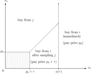
(Remember V( ) is de…ned in (1), and given this equation has a unique solution a( ).) The pattern of demand for the consumers who …rst sample …rmiis depicted in Figure 3.21

21_{This analysis and Figure 3 presume that some consumers do return to …rm i after sampling …rmj,}

which requires that the premium is not too large. By examining the …gure, one sees that the condition isa( )> p0+ . From (12), and noting thatV( )is a decreasing function, this is equivalent to < V(p0).

When the discount exceedsV(p0), the returning cost is so great that a consumer never returns to a …rm

Note that a( ) decreases with , and by di¤erentiating (12) we obtain

a0_{( ) =} F(a( ) )

1 F(a( ) ) <0 : (13)

This is intuitive, as raising the cost of returning makes a consumer more likely to buy immediately (just as in the extreme case of exploding o¤ers).

Using Figure 3, the fraction of those consumers who sample …rmi…rst and who actually buy from the …rm is

1 F(a( )) +

Z a( )

p0+

F(u )f(u)du

| {z }

…rmi’s returning consumers

:

By using (13), the derivative of …rmi’s demand with respect to is equal to

Z a( )

p0+

F(u )f0

(u)du : (14)

In particular, the …rm’s demand is boosted with a buy-later premium whenever the density is increasing, as we saw when we discussed exploding o¤ers in section 2.2.

-6 6

0 _{p0+ a( )} ui

uj

p0 buy fromi

after sampling j

(pay price p0+ )

buy fromi

immediately

(pay pricep0) buy from j

p p p p p p p p p p p p p p p p p p p p p p p p p p p p p p p p p p p p p p p p p p p p p p p p p p p p p p p p p p p p p p p p p p p p p p p p p p p p p p p p p p p p p p p p p p p p p p p p p p p p p p p p p p p p p p p p p p p p p p p p p p p p p p p p p p p p p p p p p p p p p p p

Figure 3: Pattern of demand when …rmi levies buy-later premium

Firm i makes revenue p0 from each of its customers, plus an additional from each of its customers who buy later. It follows that the derivative of …rm i’s pro…ts with respect

to evaluated at = 0 is _{Z a}

p0

Here,R_pa

0F f duis the extra revenue generated from the returning customers while

Ra p0F f

0_du

is the extra (maybe negative) demand generated by increasing the cost of return.

From (15), the …rm has an incentive to introduce a buy-now discount whenever the demand curve is concave. But it has an incentive to introduce a discount much more generally, and the incentive is present wheneverp0 in (4) is strictly above 1_fF_(a)(a), which we know from Lemma 1 is the case with strictly logconcave demand. To see this, use (4) to obtain

p0

Z a

p0

F(u)f0_{(u)du =} 1 2

p0f(a)

1 F(a)(1 F(a)

2_{) (1 F(p} 0)2)

> 1

2 F(a)

2 _F(p 0)2 =

Z a

p0

F(u)f(u)du ;

where the inequality follows from the assumption that p0 > 1_f(a)F(a). Thus, expression (15) is positive and a …rm has a unilateral incentive to o¤er a buy-now discount.

The next proposition shows that this result holds for an arbitrary number of …rms.

Proposition 4 (i) Starting from the free-recall equilibrium with pricep0 in (4), a …rm has

a unilateral incentive to o¤er …rst-time visitors a buy-now discount if the demand curve

1 F is strictly logconcave;

(ii) starting from the exploding-o¤er equilibrium with pricep in (8), a …rm has a unilateral incentive to o¤er a buy-later price low enough to induce some …rst-time visitors to return.

An implication of Proposition 4 is that if a symmetric equilibrium exists when …rms choose a buy-now and a buy-later price, it must involve an intermediate buy-now discount such that some consumers do return in equilibrium. Part (i) of Proposition 4 indicates that a seller typically has an incentive to o¤er a …rst-time visitor a discount on the regular price if the consumer buys immediately, so that uniform pricing is not an equilibrium outcome when …rms can distinguish new from returning visitors.22 _{The intuition for this result is as}

follows. As Lemma 4 shows, the impact of a small buy-now discount is the same as a small buy-later premium. A small buy-later premium has two e¤ects: the extra revenue e¤ect (every returning consumer now pays a premium) and the demand e¤ect (…rst-time visitors become more likely to buy immediately, but potential returning consumers are less likely to come back). The second e¤ect is similar to the impact of exploding o¤ers, and it is positive if the demand curve is concave. However, the …rst revenue e¤ect must be positive. Part (i) shows that this …rst e¤ect is powerful enough for the overall e¤ect to be positive under a much milder condition on the demand curve. Part (ii) shows that a …rm prefers to set a “moderate” buy-later price, rather than such a high buy-later price that none of

22_{In the example discussed in section 2.3 where match utility is exponentially distributed, a …rm does}

its initial visitors return. The intuition is that a …rm can enjoy the strategic bene…ts of exploding o¤ers but also generate some additional revenue if it charges returning visitors a high price instead of banning return altogether.23

3.2

Equilibrium buy-now discounts in duopoly

In this section we investigate the equilibrium buy-now discount in the case of duopoly.24 _We

…rst report how to derive the equilibrium prices and discuss the existence of equilibrium. We then illustrate the equilibrium outcome in the example in which match utility ui is uniformly distributed on [0;1]. For convenience, we analyze the model in terms of the buy-now price p and the buy-now discount = ^p p (rather than in terms of pand p^).

-6 6

0 _p

i + i a( i) +pi p

ui

uj

p buy from i

after samplingj (pay pi+ i)

buy from i immediately (pay pricepi)

buy from j

p p p p p p p p p p p p p p p p p p p p p p p p p p p p p p p p p p p p p p p p p p p p p p p p p p p p p p p p p p p p p p p p p p p p p p p p p p p p p p p p p p p p p p p p p p p p p p p p p p p p p p p p p p p p p p p p p p p p p p p p p p p p p p p p p p p p p p p p p p p p p p p -6 6

0 _{p+ a( )} uj

ui

pi buy fromj

after samplingi

buy from j immediately buy from i

(pay pricepi)

p p p p p p p p p p p p p p p p p p p p p p p p p p p p p p p p p p p p p p p p p p p p p p p p p p p p p p p p p p p p p p p p p p p p p p p p p p p p p p p p p p p p p p p p p p p p p p p p p p p p p p p p p p p p p p p p p p p p p p p p p p p p p p p p p p p p p p p p p p p p p p p

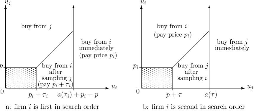
a: …rm iis …rst in search order b: …rm iis second in search order Figure 4: Pattern of demand when …rmi o¤ers(pi; i)

Suppose a symmetric equilibrium outcome is (p; )and consumers expect both …rms to o¤er this tari¤. Suppose instead that …rmideviates and o¤ers an alternative tari¤ (pi; i). It is without loss of generality that we consider deviations restricted to i V(p).25

23_{Thus, if …rms can commit to distinct prices for their …rst-time visitors and those consumers who buy}

later, we do not expect to see exploding o¤ers used in equilibrium. Nevertheless, our analysis of exploding o¤ers in section 2 is still worthwhile. For instance, the simplicity of the exploding o¤er policy may be easier to get across to consumers in a sales context, and some of the claimed “excuses” forcing quick decisions, such as the salesman being the area for that day only, make better sense for exploding o¤ers. Finally, as we discuss in section 3.3, when sellers cannot commit to their buy-later prices, exploding o¤ers emerge once more as the equilibrium sales policy.

24_{It appears to be hard to characterize the buy-now discount equilibrium for an arbitrary number of …rms,}

as we were able to do in our discussion of exploding o¤ers. As is also discussed by Janssen and Parakhonyak (2010), when there are more than two …rms the consumer stopping rule with buy-now discounts is non-stationary and depends on the history of realized match utilities, and this makes the equilibrium analysis complex. (When exploding o¤ers are used, by contrast, the stopping rule does not depend on previous o¤ers, since the consumer has no ability to return.)

25_{As can be seen from Figure 4 and expression (12), when}

Similarly to Figure 3, …rm i’s demand from those consumers who sample it …rst is as depicted on Figure 4a (they buy at …rmi immediately ifui pi > a( i) p). (Recall that

a( ) is de…ned above in (12).) Firmi’s demand from those consumers who …rst encounter the rival is shown on Figure 4b (they will come to …rm i if uj < a( ) since they hold equilibrium beliefs).

Then …rm i’s deviation pro…t is

piQT + iQR ; (16)

where QT is …rm i’s total demand and QR is the portion of demand from its returning customers. (The …rm obtains revenue pi from each of its customers, plus the incremental revenue ifrom each of its returning customers.) By calculating the measures of the regions in Figure 4 one can check that

2QT = 1 F (a( i) p+pi) +

Z a( i) i

p

F (u)f(u p+pi+ i)du

| {z }

2QR

+F(a( )) [1 F(a( ) p+pi)] +

Z a( )

p

F (u+ )f(u p+pi)du .

(The …rst line above re‡ects the demand depicted in Figure 4a, while the second line captures the demand in Figure 4b.) Using (13), one can verify that the …rst-order conditions for (p; ) to be equilibrium prices are

1 F(p)F(p+ )

p = f(a( )) +F(a( ))f(a( ) ) (17)

Z a( )

p

F(u+ )f0

(u) + (1 +

p)F(u)f

0

(u+ ) du ;

and

f(a( ))F(a( ) )

1 F(a( ) ) =

Z a( )

p

F(u)[(p+ )f0

(u+ ) +f(u+ )]du : (18) If = 0, expression (17) degenerates to the …rst-order condition (4) in Wolinsky’s model withn= 2. If =V(p)(i.e., p=a( ) ) so there are no returning consumers, expression (17) degenerates to the …rst-order condition (8) in the exploding-o¤er regime with n = 2. In particular, when u is uniformly distributed on [0;1], so that a( ) = 1 p2(s+ )

and s < 1₈, the above two …rst-order conditions become

1

p p= 1 +a( ) + ;

2 [a( ) ]

1 a( ) + = [a( ) ]

2 _p2 _:

In our online appendix, we show that under some conditions (e.g., when the density function

existence of returning consumers in equilibrium), and in the uniform example, the …rst-order conditions are also su¢cient for (p; ) to be the equilibrium prices.

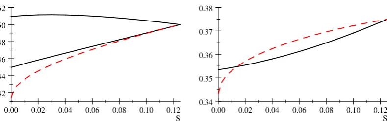
In the following, we report some properties of the uniform example. First, as with the use of exploding o¤ers in Proposition 3, we observe that the use of buy-now discounts leads to higher prices, i.e., p0 < p < p^. That is, even the discounted buy-now price in the discriminatory case is higher than the uniform price, and the ability to o¤er such discounts drives up both prices.26 _{The intuition is that the buy-now discount adds to the intrinsic}

search frictions in the market, and this allows …rms to charge a higher price. Figure 5a below depicts how the three prices vary with the search cost s, where from the bottom up the three curves represent p0, p and p^, respectively.

Second, the equilibrium buy-now discount (the distance between the upper curve and the middle curve in Figure 5a) decreases with the search costs. In particular, when s= 0, we havep 0:45and p^ 0:51, and so 0:06. In this case, although the market has no intrinsic search frictions, …rms in equilibrium generate search frictions on consumers via the buy-now discount, which here is about 12% of the buy-later price. By contrast, in a market with s = 1₈, which is the highest intrinsic search cost which induces consumers to participate, we have p = ^p = 1₂ and = 0, so that there is no buy-now discount. (When

s = 1₈, search costs are so high that consumers will accept the …rst o¤er which yields a non-negative surplus. In particular, there are no returning consumers even with costless recall.)

0.00 0.02 0.04 0.06 0.08 0.10 0.12 0.42

0.44 0.46 0.48 0.50 0.52

s

Figure 5a: Prices and search cost

0.00 0.02 0.04 0.06 0.08 0.10 0.12 0.34

0.35 0.36 0.37 0.38

s

Figure 5b: Pro…ts and search cost

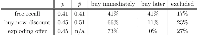
Since both prices rise, the buy-now discount equilibrium excludes more consumers from the market. In addition, as expected, the use of buy-now discounts boosts the demand from consumers who buy immediately and reduces demand from those who buy later. This is illustrated for the cases= 0in Table 1 (including for reference the case where exploding o¤ers are used).

26_{It is not unusual that the ability to price discriminate in oligopoly leads to a fall in all prices, but cases}

p p^ buy immediately buy later excluded

free recall 0.41 0.41 41% 41% 17%

buy-now discount 0.45 0.51 66% 11% 23%

exploding o¤er 0.45 n/a 73% 0% 27%

Table 1: The impact on prices and demand of buy-now discounts and exploding o¤ers

However, whether the use of buy-now discounts leads to higher pro…t depends on the magnitude of the search cost. Figure 5b shows how industry pro…ts with uniform pricing (the dashed curve) and pro…ts with buy-now discounts (the solid curve) vary with the search costs. We see that price discrimination leads to higher pro…t only if the search cost is relatively small. When the search cost is relatively high, price discrimination leads to prices which exclude too many consumers. In these cases, …rms are engaged in a prisoner’s dilemma: when feasible an individual …rm wishes to o¤er a buy-now discount, but when both do so industry pro…ts fall. Finally, for similar reasons as in the exploding-o¤er case, aggregate consumer surplus and total welfare fall when …rms use buy-now discounts in this example.

3.3

Buy-later prices without commitment

The preceding analysis has assumed that a …rm can commit to its buy-later price when consumers …rst visit. We discuss here whether buy-now discounts are used if we relax this assumption. That is to say, we investigate whether …rms wish to implement an unan-nounced price rise when consumers return to buy. The basic game structure is the same as before, except that now when a consumer discovers a …rm’s buy-now price, she can only form some belief about its buy-later price (the belief is of course required to be correct in equilibrium). The actual buy-later price can be learned only after she returns to the …rm. Here, unlike the rest of the paper, it makes an important di¤erence whether or not consumers face an intrinsic returning cost when they come back to a previously-visited …rm. Since in most situations such a returning cost does exist, we focus on this case. (In the previous analysis with commitment, the presence of a small intrinsic return cost makes no qualitative di¤erence, and for simplicity we assumed this cost was precisely zero.) Proposition 5 describes the outcome when …rms cannot fully commit to their buy-later price.27

27_{If, by contrast, consumers face no intrinsic returning cost, there is often an equilibrium in which}

Proposition 5 Suppose consumers face an intrinsic returning cost.

(i) If …rms cannot commit to their buy-later price, in equilibrium no consumers return to a previously-visited …rm and the equilibrium price is as described in Lemma 3;

(ii) if …rms can commit to an upper bound on their buy-later price, then …rms in any equilibrium will choose their buy-later price to equal the upper bound, and the outcome is as if …rms can fully commit to their buy-later prices.

Thus, part (i) shows that if …rms cannot commit to their buy-later price and if there is an intrinsic returning cost (no matter how small), rational consumers anticipate that buy-later prices will be so high that it is never worthwhile to return to a previous …rm after leaving it. In e¤ect, because of the informational motive to raise prices to those consumers who buy later, …rms are forced to make exploding o¤ers, and consumers have just one chance to buy from any …rm. Thus, the lack of commitment power strengthens a …rm’s temptation to exploit returning consumers. This result is analogous to Diamond’s (1971) paradox, showing how a small search cost can cause a market to shut down. Diamond’s result relies on consumers knowing their match utility in advance, and a central advantage of Wolinsky’s formulation with ex ante unknown match utilities is that this paradox can be avoided. But even in Wolinsky’s framework, thereturning consumers know their match utilities, and so the returning market fails for the same reason as the primary market failed in Diamond’s framework.

Of course, as shown in part (ii) of Proposition 4, a …rm would like to avoid this complete shut down of the return market if possible. One method, when feasible, is to commit to a buy-later price cap. For instance, in most retailing markets the price printed on the price label in the store usually has this commitment power, and a sales person has no authority to increase the price above the displayed price. Similarly, as discussed in the introduction, the …rm in Bone’s (2006) study o¤ered its potential customers a regular price (in the form of a written quote) if they decided to buy later. Whenever this form of partial commitment is feasible, part (ii) of Proposition 5 shows that the equilibrium is the same as that in the full commitment situation analyzed in sections 3.1 and 3.2. Thus, a cap on the buy-later price can be used as a full commitment device.

4

Alternative Motives for Exploding O¤ers

Factors other than those discussed in our main model may also play a role in giving …rms an incentive to use high-pressure sales tactics, and in this section we discuss additional motivations for making exploding o¤ers.

model with zero search costs, and the incentive to set the price to returning consumers is exactly the same as the incentive to set the uniform pricep0in thes= 0version of expression (4). If search is costly (s >0)

4.1

Exploding o¤ers with homogenous products

The analysis to this point has used Wolinsky’s framework with di¤erentiated products and no equilibrium price dispersion. In many search markets, however, consumers do not face signi…cant uncertainty about the utility they obtain from a seller’s product, but rather from the price they will pay. In this alternative situation, does a seller also have an incentive to use an exploding o¤er? We explore this issue in the context of Stahl’s (1989) model with homogenous products and endogenous price dispersion.

Consider Stahl’s model with n …rms and unit consumer demand. Let v be each con-sumer’s willingness to pay for the product. All consumers are risk neutral and sample …rms sequentially and randomly to gather price information. A fraction of consumers are “shoppers” who have zero search cost (so they will be fully informed of market prices if sellers put no restrictions on their ability to return to a previously sampled …rm), and a fraction 1 of consumers have a positive search cost s > 0 for sampling an additional …rm. (These costly searchers are assumed to be able to sample the …rst …rm for free.) Stahl’s model assumed free recall, so that each …rm allowed consumers to return to buy after they have investigated its rivals. As explained by Stahl, in equilibrium …rms choose prices according to a mixed strategy, and there is price dispersion in the market. In more detail, in symmetric equilibrium each …rm chooses its price according to a c.d.f. G(p)with support[pmin; r], the shoppers investigate all sellers and buy from the cheapest seller, while the costly searchers stop searching whenever they …nd a price no greater than r and so buy from the …rst …rm they encounter.28 _{In order for a …rm to be indi¤erent between all}

prices in the interval [pmin; r], a …rm’s pro…t must be constant in this range.

Starting from Stahl’s free-recall equilibrium, we show that a …rm always has a strict incentive to make an exploding o¤er. This stands in contrast to the more ambiguous situation with product di¤erentiation (see Proposition 1 above). This result is relatively easy to understand in the case of duopoly. Suppose that one …rm is considering whether to make an exploding o¤er at some pricep₂[pmin; r], given that its rival allows free recall and charges a stochastic price according to the c.d.f. G( ). A costly searcher will buy from the …rm (given p r), regardless of whether it makes an exploding o¤er or not. Likewise, those shoppers who …rst encounter the rival seller will be una¤ected by the …rm’s use of an exploding o¤er. Thus, to determine whether making an exploding o¤er is pro…table for the …rm, we need only consider its demand from those shoppers who visit it …rst. If the …rm sets price p ₂ (pmin; r) and allows free recall, it competes against a rival o¤ering a stochastic price and so will make the sale with probability less than one. (Recall that each such price generates the same expected pro…t in the free-recall equilibrium.) If it instead uses an exploding o¤er, it competes against a rival o¤ering the (known) expected price

p=R_pr

minpdG~ (~p). Hence, using an exploding o¤er with any price in the range pmin < p < p

28_{A costly searcher’s reservation price ris endogenously determined in equilibrium. (When the search}