Fast Tensor Principal Component Analysis via Proximal Alternating Direction Method with Vectorized Technique

(1)

http://www.scirp.org/journal/am ISSN Online: 2152-7393

ISSN Print: 2152-7385

Fast Tensor Principal Component Analysis via

Proximal Alternating Direction Method with

Vectorized Technique

Haiyan Fan1_{, Gangyao Kuang}1_{, Linbo Qiao}2

1_{Department of Electronic Science and Engineering, National University of Defense Technology, Changsha, China} 2_{Department of Computer, National University of Defense Technology, Changsha, China}

Abstract

This paper studies the problem of tensor principal component analysis (PCA). Usually the tensor PCA is viewed as a low-rank matrix completion problem via matrix factorization technique, and nuclear norm is used as a convex ap-proximation of the rank operator under mild condition. However, most nuc-lear norm minimization approaches are based on SVD operations. Given a matrix ∈ m n×

X  , the time complexity of SVD operation is

( )

2

O mn , which

brings prohibitive computational complexity in large-scale problems. In this paper, an efficient and scalable algorithm for tensor principal component analysis is proposed which is called Linearized Alternating Direction Method with Vectorized technique for Tensor Principal Component Analysis (LADMVTPCA). Different from traditional matrix factorization methods, LADMVTPCA utilizes the vectorized technique to formulate the tensor as an outer product of vectors, which greatly improves the computational efficacy compared to matrix factorization method. In the experiment part, synthetic tensor data with different orders are used to empirically evaluate the proposed algorithm LADMVTPCA. Results have shown that LADMVTPCA outper-forms matrix factorization based method.

Keywords

Tensor Principal Component Analysis, Proximal Alternating Direction Method, Vectorized Technique

1. Introduction

A tensor is a multidimensional array. For example, a first-order tensor is a vec-tor, a second-order tensor is a matrix, and tensors with three or higher-order are How to cite this paper: Fan, H.Y., Kuang,

G.Y. and Qiao, L.B. (2017) Fast Tensor Principal Component Analysis via Proxim-al Alternating Direction Method with Vec-torized Technique. Applied Mathematics, 8, 77-86.

http://dx.doi.org/10.4236/am.2017.81007

Received: November 12, 2016 Accepted: January 21, 2017 Published: January 24, 2017

(2)

called higher-order tensors. Principal component analysis (PCA) finds a few li-near combinations of the original variables. The PCA plays an important role in dimension reduction and data analysis related research areas [1]. Although the PCA and eigenvalue problem for the matrix has been well studied in the litera-ture, little work has been done on the study of tensor PCA analysis.

The tensor PCA is of great importance in practice and has many applications, such as computer vision [2], social network analysis [3], diffusion Magnetic Re-sonance Imaging (MRI) [4] and so on. Similar to its matrix form, the problem of finding the PCs is related to the most variance of a tensor  , which can be

specifically formulated as [5]:

1 2

2 1 2

,min, , ,

, 1, 1, 2, , ,

m

m F

x x x

i

x x x

st x i m

λ

− ⊗ ⊗ ⊗

∈ = =

 

 



(1)

which is equivalent to

(

)

1 2

1 2 , , ,

min ,

1, 1, 2, , ,

m

x x x

i

x x x

st x i m

− ⋅ ⊗ ⊗ ⊗

= =

 

 

(2)

where ⋅ denotes the inner product between two tensors, and the inner product of two tensors 1 2

1, 2 m

n n× × ×n

∈_ 

  is denoted as

( )

1 2 1 2 1 2

1⋅ 2 =

∑

i i, , ,i_m 1 i ii_m 2 i ii_m.

    (3)

And ⊗_{denotes the outer product between vectors, i.e.}_[6]_[7]_:

(

)

( )

1 2

=1

= .

m k

m

m k

k

i i i i

x ⊗x ⊗ ⊗x

∏

x



 (4)

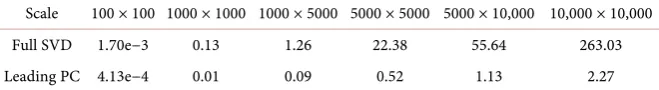
[image:2.595.208.538.687.732.2]

The above solution is called the leading PC. Once the leading PC is found, the other PCs can be computed sequentially via the so-called deflation technique. For example, the second PC could be gotten in the following ways: 1) Generate the first leading PC of the tensor, 2) Subtract the first leading PC of the tensor from the original tensor, 3) Generate the leading PC of the rest tensor. This leading PC is noted as the second PC of the original Tensor. And the rest PCs could be obtained in a similar way [8][9]. The deflation procedure is presented in Algorithm 1. Although theoretical analysis of deflation procedure for matrix is well established (see [10] and the references therein for more details), the ten-sor counterpart has not been completely studied. However, the deflation process does provide an efficient heuristic way to compute multiple principal compo-nents of a tensor. The time consumption of different scaled between full SVD and leading PC is shown in Table 1. When the size of matrix increases, the computational cost for leading PC is far less than that of full SVD. Therefore,

Table 1. The comparison of running time (seconds) between full SVD and leading PC. Scale 100 × 100 1000 × 1000 1000 × 5000 5000 × 5000 5000 × 10,000 10,000 × 10,000 Full SVD 1.70e−3 0.13 1.26 22.38 55.64 263.03

(3)

although more iterations are needed for greedy atom decomposition methods to reach convergence, their total computational costs are much less compared with SVD based matrix completion methods. Thus, in the rest of this paper, we focus on finding the leading PC of a tensor.

If  is a super-symmetrical tensor, problem (2) can be reduced to [9]

(

)

min ,

1.

x x x x

st x

− ⋅ ⊗ ⊗ ⊗ =

 

(5)

In fact, the algorithm for supersymmetric tensor PCA problem can be ex-tended to tensors that are not super-symmetric [5]. Therefore, this paper focuses on the PCA analysis of super-symmetric tensors. Problem (5) is NP-hard and is known as the maximum Z-eigenvalue problem. Note that a variety of eigenva-lues and eigenvectors of a real symmetric tensor were introduced by Lim [11]

and Qi [9] independently in 2005. Since then, various methods have been pro-posed to find the Z-eigenvalues, which however may correspond only to local optimums.

Another research line, like CANDECOMP (canonical decomposition) and PARAFAC (parallel factors) propose imposing rank-one constraint of tensor to realize the tensor decomposition:

( )

1 2

, 1 2

1

min ,

!

1, !

rank 1,

k k k n

m n

k n m n

j j

n

m st

k ∈

=

− ⋅

=

= ∈

∑

∏





 



  

(6)

where  = ⊗ ⊗x x ⊗x and

(

)

{

(

₁

)

}

1

, , , m n

n j j

n m = k= k  k ∈₊

∑

₌k =m

 .

)

=1, ∈ nm

   indicates that  should be super-symmetrical. The first equality constraint is due to the fact that ( , ) 1 21 2

1

!

1 ! k k kn

d n

k n m n

j j m

x k

∈

=

= =

∑

∏



  .

The difficulty of problem (6) lies in the dealing of the rank constraint

( )

rank  =1. Not only the rank function itself is difficult to deal with, but also determining the rank of a specific given tensor is already a difficult task, which is NP-hard in general. One way to deal with the difficulty is to convert the tensor optimization problem into a matrix optimization problem. [5] proved that if the tensor is rank-one, then the embedded matrix must be rank-one too, and vice versa. The tensor PCA problem can thus be solved by means of matrix optimiza-tion under a rank-one constraint. For low-rank matrix optimizaoptimiza-tion problem, a nuclear norm penalty is often adopted to enforce a low-rank solution. However, most nuclear norm minimization approaches are based on SVD operations. Given a matrix _∈ m n×

X  , the time complexity of SVD operation is O mn

( )

2 , which will bring prohibitive computational complexity in large problems (refer to Table 1).

(4)

( )

(

)

1 2

, , ,

1 2

min Vec Vec ,

1, 1, 2, , ,

m

m x x x

i

m

x x x

st x i m

x x x

− ⋅ ⊗ ⊗ ⊗

= =

= = =

 



(7)

where Vec

( )

 is the vectorized form of tensor  . Related stream of

algo-rithms to solve problem (7) are the ADM-type algoalgo-rithms [12][13]. Such a kind of algorithms has recently been shown effective to handle some non-convex op-timization problems [14] [15]. However, the results of [14] require a lot well-justified assumption. Besides, the subproblems in ADM are easily solvable only when the linear mappings in the constraints are identities. To address this issue, [16] proposed a linearized ADM (LADM) method by linearizing the qua-dratic penalty term and adding a proximal term when solving the subproblems. In this paper, we adopt LADM algorithm for solving the optimization problem (7).

The rest of this paper is organized as follows. In Section 2, a brief review of LADM algorithm is firstly given. And then, the detailed description of using LADM with vectorized technique to solve tensor principal component problem is presented. Section 3 is the experiment part, in which synthetic tensor data with different orders are used to empirically evaluate the proposed algorithm LADMVTPCA. The last section gives concluding remarks.

Algorithm 1 Deflation Procedure

Input: _{Σ = ∅}0 , 0

V = ∅, _0₌_

Output: Σ, V

Initialization: Setup parameters while (True) do

Update λk+1 and k1

x+ by solving (7)

Update k1 k k1

x

+ +

Σ = Σ ∪ , Update k1 k k1

V + =V ∪λ+ ,

Update k1 k k1 k1 k1

x x

λ

+ ₌ ₋ + + _⊗ +

  ,

1

k= +k ,

if (stopping criteria satisfied) then Break.

end if end while

2. Linearized Alternating Direction Method (LADM)

In this section, we first review the Linearized Alternating Direction Method of Multipliers (LADM) [16], and then we present the linearized ADM for solving tensor principal component problem.

2.1. Algorithm

Considering the convex optimization problem,

( ) ( )

,

min ,

. . 0.

x y l x r y

s t Ax By

+

− = (8)

where d

x∈ , _y∈_l, _A_∈_p d× , _B_∈_p l× , and p

(5)

that problem (8) can be solved by the standard ADMM with typical iteration written as

(

)

1

: arg min , , ,

k k k

x

x+ = β x y λ (9)

(

)

1 1

: ,

k k k k

Ax By

λ + ₌λ ₋β + ₋

(10)

(

)

1 1 1

: arg min , , ,

k k k

y

y + = β x + y λ + (11)

where the augmented Lagrangian function β

(

x y, ,λ

)

is defined as

(

) ( ) ( )

2

, , , .

2

x y l x r y Ax By Ax By

β λ = + − λ − +β −

 (12)

The penalty parameter β >0 is a constant dual step-size. The inefficient of ADMM inspires a linearized ADMM algorithm [16] by linearizing l x

( )

in the

x-subproblem. Specifically, it considers a modified augmented Lagrangian

function:

(

) ( )

( )

2

ˆ ˆ ˆ ˆ

, , , ,

, .

2

x x y l x l x x x r y

Ax By Ax By

β λ

= + ∇ − +

− − + −



(13)

Then the LADM algorithm solves problem (8) by generating a sequence

{

1 1 1

}

, ,

k k k

x+ λ + z + as follows:

(

)

1

: arg min , , , ,

k k k k

x

x + = β x x y λ (14)

(

)

1 1

: ,

k k k k

Ax By

λ + ₌λ ₋β + ₋ ₍₁₅₎

(

)

1 1 1

: arg min , , , .

k k k k

y

y + = β x + x yλ + (16)

The framework of linearized ADMM is given in Algorithm 2.

Algorithm 2 LADM

Choose the parameter β such that Equation (9) is satisfied;

Initialize an iteration counter k←0 and a bounded starting point

(

x0,λ0,y0

)

; repeat

Update k1

x+ according to Equation (14);

(

)

1 1

k k _Axk _Byk

λ+ _←λ ₋β + ₋

;

Update _yk+1_{according to Equation (16);} if some stopping criterion is satisfied; then

Break; else

1

k← +k ; end if

until exceed the maximum number of outer loop.

2.2. Linearized ADM with Vectorized Technique

(6)

prob-lem (17).

( )

(

)

, ,

2

2 2 2 2

min Vec Vec ,

. . , , ,

1, 1, 1, 1.

x y z x y z w

s t x y y z z w

x y z w

− ⋅ ⊗ ⊗ ⊗

= = =

= = = =



(17)

where x y z w, , , are variables updated from iteration to iteration, the constraints , ,

x= y y=z z=w limite the variables are close to each other and finally overlap,

and the constraints 2

2 1, 1, 1, 12 2 2

x = y = z = w = make the solution

ro-bust to the scaling. After adding the constraints into the loss function, the prob-lem (17) is equivalently reformed as

( )

(

)

(

)

1 , ,

2 3 4

2 2 2 2

min Vec Vec ,

, , ,

,

2

. . , , , ,

x y z x y z w x y

y z z w w x

x y y z z w w x

s t x y z w

λ

λ λ λ

ρ

− ⋅ ⊗ ⊗ ⊗ + −

+ − + − + −

+ ∗ − + − + − + −

∈ 



(18)

where =

{

x x 2=1

}

is a unit ball and ρ is a parameter to balance the

ob-ject loss and the smooth terms. It should be noted that tensors with different or-ders could be deduced in a similarly way. The augmented Lagrangian function

(

x y z w, , , ,λ λ λ λ ρ1, 2, 3, 4,

)

 is defined as

(

)

( )

(

)

(

)

1

2 3 4

2 2 2 2

, , , ,

: Vec Vec ,

, , ,

.

2 x y z w

x y z w x y

y z z w w x

x y y z z w w x

ρ

λ

λ λ λ

ρ

= − ⋅ ⊗ ⊗ ⊗ + −

+ − + − + −

+ ∗ − + − + − + −





(19)

where x y z w, , , ∈. In the k-th iteration, we denote the variables by , , ,

k k k k

x y z w , and ρk. Given xk,yk,zk,wk,ρk, iterates as follows Algorithm 3 Algorithm for solving program (18)

Input: 0

x , y0, 0 z , 0

w , ρ0 Output: x, y, z, w Initialization: Setup parameters while (Stop == False) do

Update k1

x+ by solving (20a) Update _yk+1_{by solving (20b),} Update k1

z+ by solving (20c), Update k1

w+ by solving (20d), Update λ λ λ λ1, 2, 3, 4,

Update ρk+1_{by (20f),}

1

k= +k ,

if Stopping condition satisfied then

Stop = True end if end while

(

)

1

: arg min , , , , ,

k k k k k

x

x+ x y z w ρ

∈

=

(7)

(

)

1_{: arg min} 1_{, ,} _, _, _,

k k k k k

y

y+ x+ y z w ρ

∈

=

  (20b)

(

)

1_{: arg min} 1_, 1_{, ,} _, _,

k k k k k

z

z+ x+ y + z w ρ

∈

=

  (20c)

(

)

1 1 1 1

: arg min , , , , ,

k k k k k

w

w+ x + y+ z+ w ρ

∈

=

  (20d)

1 2 3 4

Update ,λ λ λ λ, , (20e)

1 Balancedcases : Others. k k k αρ ρ ρ α + _{= }

 (20f)

In the following part, we show how to solve these subproblems in the algo-rithm through a linearized way with vectorized technique. After all these sub-problems solved, we will give the framework of the algorithm that summarize our algorithm for solving (18) in Algorithm 3. In order to achieve the saddle fast and improve the quality of the solution, we adjust the parameter ρ adaptively to balance the decrease speed of these two parts.

In a traditional way, k 1

x + is obtained by minimizing  with respect to

va-riable x while y z w, , ,ρ are fixed with the value k, k, k, k

y y w ρ respectively,

and the Lagrange function is put forward as follow:

( )

(

)

(

)

1

2 3 4

2 2 2 2

: arg min Vec Vec ,

, , ,

.

2

k k k k k

x

k k k k k

k k k k k k

x x y z w x y

y z z w w x

x y y z z w w x

λ

λ λ λ

ρ + ∈ = − ⋅ ⊗ ⊗ ⊗ + − + − + − + − + ∗ − + − + − + −   (21)

We slightly modify the above LADM algorithm by imposing a proximal term

2

k

x x

δ ₋

on the subproblem of x and update xk+1 via

( )

(

)

(

)

1

2 3 4

2 2 2 2

2

: arg min Vec Vec ,

, , ,

2

.

2

k k k k k

x

k k k k k

k k k k k k

k

x x y z w x y

y z z w w x

x y y z z w w x

x x

λ

λ λ λ

ρ δ + ∈ = − ⋅ ⊗ ⊗ ⊗ + − + − + − + − + ∗ − + − + − + − + −   (22)

The minimum value will be obtained while the derivative of  with respect

to x setting to zero, and utilize this condition, we obtain an equation which

implies the solution of the subproblem

( )

(

)

(

)

(

)

1 4

0 Vec Vec ,

2 .

k k k

k k k k

y z w x

x x x y w

λ λ δ ρ ∈ ⋅ ⊗ ⊗ + − + − + − −  (23)

where Vec

( )

 is the vectorized form of tensor  , after solving the above equation, we get the k 1

x + . For parsimony purpose, we just present the solving of

the first subproblem here.

3. Numerical Experiments

(8)

3 to solve the tensor leading PC problem (18). As the ADMPCA [5] is one of these fastest methods based on matrix factorization and outperforms the SVD based methods, we will mainly focus on the comparison of our approach with ADMPCA proposed in [5]. The MATLAB codes of ADMPCA were downloaded from Professor Shiqian Ma’s [5] homepage.

We apply our approach to synthetic datasets. The data is generated with uni-form distributed eigen vectors xi and eigen value λi, and the tensor is

gener-ated through the summation 1

n

i i i i

i=λ v v v

=

∑

∗ ⊗ ⊗

 , in which the rank of

tensor is controlled by the number of eigen vectors n, the order of tensor is

controlled by number of vi appear in the outer product, and the dimension of

tensor is controlled by the dimension of the vector vi.

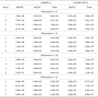
We compare LADMVTPCA with ADMPCA for solving problem (18). In Ta-ble 2, we report the results on randomly created tensor with order=4 and

dimension=4,8,16, 32. “objDiff” is used to denote the relative difference of the solutions obtained by ADMPCA and LADMVTPCA,

{

}

LADMVTPCA ADMPCA

ADMPCA

objDiff

max 1,

F F

−

=  

 . “objVal” is used to denote the relative

dif-ference of the objective eigen vectors, LADMVTPCA

_{

ADMPCA

_}

ADMPCA

objVal

max 1,

F F

v v

v

−

[image:8.595.206.539.405.735.2]

= _{. “Time”}

Table 2. Results of different algorithms for solving randomly generated tensor’s leading principal component.

ADMPCA LADMVTPCA

Inst.# objDiff. objVal Time objVal Time

Dimension n = 4

1 2.92e−06 1.07e+02 6.62e-01 1.07e+02 2.00e−03 2 7.29e−04 1.00e+02 6.57e-01 1.00e+02 3.01e−03 3 3.73e−04 1.00e+02 7.02e-01 1.00e+02 1.01e−03 4 4.57e−05 1.00e+02 6.85e-01 1.00e+02 1.92e−03

Dimension n = 8

1 2.64e−06 1.00e+02 4.55e+00 1.00e+02 3.01e−03 2 1.66e−08 1.00e+02 4.48e+00 1.00e+02 3.00e−03 3 1.58e−05 1.00e+02 4.16e+00 1.00e+02 3.00e−03 4 1.32e−07 1.00e+02 4.42e+00 1.00e+02 3.00e−03

Dimension n = 16

1 2.89e−04 1.04e+02 4.45e+01 1.04e+02 1.10e−02 2 2.13e−07 1.00e+02 4.65e+01 1.00e+02 7.00e−03 3 1.29e−05 1.00e+02 4.61e+01 1.00e+02 1.30e−02 4 2.63e−07 1.00e+02 4.64e+01 1.00e+02 1.18e−02

Dimension n = 32

(9)

denote the CPU times (in seconds) of ADMPCA and LADMVTPCA, respec-tively. From Table 2 we can see that, LADMVTPCA produced comparable solu-tions compared to ADMPCA; however, LADMVTPCA was much faster than ADMPCA, especially for large-scale problem, i.e. n = 16, 32. Note that when n = 16, LADMVTPCA was about 4000 times faster than ADMPCA.

4. Conclusion

Tensor PCA is an emerging area of research with many important applications in image processing, data analysis, statistical learning, and bio-informatics. In this paper, we propose a new efficient and scalable algorithm for tensor principal component analysis called LADMVTPCA. A vectorized technique is introduced in the processing procedure and linear alternating direction method is used to solve the optimization problem. LADMVTPCA provides an efficient way to com-pute the leading PC. We empirically evaluate the proposed algorithm on synthetic tensor data with different orders. Results have shown that LADMVTPCA has much better computational cost beyond matrix factorization based method. Es-pecially for large-scale problems, matrix factorization based method is much more time-consuming than our method.

References

[1] Kolda, T.G. and Bader, B.W. (2009) Tensor Decompositions and Applications. SIAM Review, 51, 455-500.https://doi.org/10.1137/07070111X

[2] Wang, H. and Ahuja, N. (2004) Compact Representation of Multidimensional Data Using Tensor Rank-One Decomposition. Proceedings of the 17th International Conference on Pattern Recognition, ICPR 2004, Cambridge, 26-26 August 2004, 104-107.

[3] Huang, F., Niranjan, U., Hakeem, M.U. and Anandkumar, A. (2013) Fast Detection of Overlapping Communities via Online Tensor Methods. arXiv:1309.0787

[4] Qi, L., Yu, G. and Wu, E.X. (2010) Higher Order Positive Semidefinite Diffusion Tensor Imaging. SIAM Journal on Imaging Sciences, 3, 416-433.

https://doi.org/10.1137/090755138

[5] Jiang, B., Ma, S. and Zhang, S. (2014) Tensor Principal Component Analysis via Convex Optimization. Mathematical Programming, 1-35.

[6] Hitchcock, F.L. (1927) The Expression of a Tensor or a Polyadic as a Sum of Prod-ucts. Journal of Mathematics and Physics, 6, 164-189.

[7] Kofidis, E. and Regalia, P.A. (2002) On the Best Rank-1 Approximation of High-er-Order Supersymmetric Tensors. SIAM Journal on Matrix Analysis and Applica-tions, 23, 863-884.https://doi.org/10.1137/S0895479801387413

[8] Kolda, T.G. and Mayo, J.R. (2011) Shifted Power Method for Computing Tensor Eigenpairs. SIAM Journal on Matrix Analysis and Applications, 32, 1095-1124.

https://doi.org/10.1137/100801482

[9] Qi, L. (2005) Eigenvalues of a Real Supersymmetric Tensor. Journal of Symbolic Computation, 40, 1302-1324.https://doi.org/10.1016/j.jsc.2005.05.007

[10] Mackey, L.W. (2009) Deflation Methods for Sparse PCA. Advances in Neural In-formation Processing Systems, 21, 1017-1024.

(10)

Ap-proach. IEEE International Workshop on Computational Advances in Multi-Sensor Adaptive Processing, Puerto Vallarta, Mexico, 13-15 December 2005, 129-132. [12] Zhong, L.W. and Kwok, J.T. (2013) Fast Stochastic Alternating Direction Method of

Multipliers. Proceedings of the 30th International Conference on Machine Learn-ing, Atlanta, Georgia, 2013.

[13] Zhao, P.l., Yang, J.W., Zhang, T. and Li, P. (2013) Adaptive Stochastic Alternating Direction Method of Multipliers.arXiv:1312.4564

[14] Magnússon, S., Weeraddana, P.C., Rabbat, M.G. and Fischione, C. (2014) On the Convergence of Alternating Direction Lagrangian Methods for Nonconvex Struc-tured Optimization Problems. arXiv:1409.8033 [math.OC]

[15] Hong, M.Y., Luo, Z.-Q. and Razaviyayn, M. (2015) Convergence Analysis of Alter-nating Direction Method of Multipliers for a Family of Nonconvex Problems. 2015 IEEE International Conference on Acoustics, Speech and Signal Processing (ICASSP), Brisbane, 19-24 April 2015, 3836-3840.

https://doi.org/10.1109/ICASSP.2015.7178689

[16] Yang, J. and Yuan, X. (2013) Linearized Augmented Lagrangian and Alternating Direction Methods for Nuclear Norm Minimization. Mathematics of Computation, 820, 301-329.

Submit or recommend next manuscript to SCIRP and we will provide best service for you:

Accepting pre-submission inquiries through Email, Facebook, LinkedIn, Twitter, etc. A wide selection of journals (inclusive of 9 subjects, more than 200 journals)

Providing 24-hour high-quality service User-friendly online submission system Fair and swift peer-review system

Efficient typesetting and proofreading procedure

Display of the result of downloads and visits, as well as the number of cited articles Maximum dissemination of your research work