Effect of spatial distribution of daily rainfall on interior catchment response of a distributed hydrological model

www.hydrol-earth-syst-sci.net/11/677/2007/ © Author(s) 2007. This work is licensed under a Creative Commons License.

Earth System

Sciences

Effect of spatial distribution of daily rainfall on interior catchment

response of a distributed hydrological model

J. M. Schuurmans1and M. F. P. Bierkens1,2

1_{Department of Physical Geography, Faculty of Geosciences, Utrecht University, P.O. Box 80115, 3508 TC, Utrecht, The} Netherlands

2_{TNO Built Environment and Geosciences, P.O. Box 80015, 3508 TA Utrecht, The Netherlands} Received: 26 June 2006 – Published in Hydrol. Earth Syst. Sci. Discuss.: 9 August 2006 Revised: 20 November 2006 – Accepted: 13 December 2006 – Published: 17 January 2007

Abstract. We investigate the effect of spatial variability of daily rainfall on soil moisture, groundwater level and dis-charge using a physically-based, fully-distributed hydrolog-ical model. This model is currently in use with the district water board and is considered to represent reality. We focus on the effect of rainfall spatial variability on day-to-day vari-ability of the interior catchment response, as well as on its ef-fect on the general hydrological behaviour of the catchment. The study is performed in a flat rural catchment (135 km2) in the Netherlands, where the climate is semi-humid (average precipitation 800 mm/year, evapotranspiration 550 mm/year) and rainfall is predominantly stratiform (i.e. large scale). Both range-corrected radar data (resolution 2.5×2.5 km2) as well as data from a dense network of 30 raingauges are used, observed for the period March–October 2004. Eight differ-ent rainfall scenarios, either spatially distributed or spatially uniform, are used as input for the hydrological model. The main conclusions from this study are: (i) using a single rain-gauge as rainfall input carries a great risk for the prediction of discharge, groundwater level and soil moisture, especially if the raingauge is situated outside the catchment; (ii) taking into account the spatial variability of rainfall instead of using areal average rainfall as input for the model is needed to get insight into the day-to-day spatial variability of discharge, groundwater level and soil moisture content; (iii) to get in-sight into the general behaviour of the hydrological system it is sufficient to use correct predictions of areal average rain-fall over the catchment.

1 Introduction

Rainfall is often defined as being the key variable in hy-drological systems. Considering the question how the

spa-Correspondence to: J. M. Schuurmans

([email protected])

tial variability of rainfall influences the hydrological state, most studies have focussed on the effect on catchment dis-charge (e.g. Obled et al., 1994; Arnaud et al., 2002; Bell and Moore, 2000; Shah et al., 1991). Obled et al. (1994) conclude from their study (using TOPMODEL for a rural catchment of 71 km2) that the spatial variability must be taken into account more because it improves the estimation of the basin aver-age incoming volume, rather than because of some dynamic interactions with flow-generating processes. Arnaud et al. (2002) (using 3 different rainfall-runoff models for 4 ficti-tious catchments of 20–1500 km2) however, found that rain-fall variability can lead to significant different discharge, not for extreme events but for the more frequent events. This was also concluded by Shah et al. (1991): under “wet” conditions, good predictions of runoff can be obtained with a spatially averaged rainfall input but under “dry” conditions, spatial variability of rainfall has a significant influence. They sug-gest this is caused by the spatial distribution of soil moisture which controls the runoff production. Bell and Moore (2000) also show the importance of taking into account the spatial variability of rainfall, especially in case of convective rain-fall events, which show high spatial variability. O’Connell and Todini (1996) point out the need to study the influence of space-time rainfall variability on the hydrological system in real catchments, but up to now not much attention has been given to the influence of rainfall variability on groundwater level and soil moisture content within the catchment.

to be uniform in the application of hydrological models of small catchments. This is also the case in the Netherlands where often data from a single raingauge (even outside the catchment area) is used as input for hydrological model stud-ies.

The main objective of our study is to determine how spatial variability of daily rainfall affects soil moisture, groundwa-ter level and discharge as calculated by a physically-based, fully-distributed hydrological model. This is done for 2 pur-poses. First, to assess the effect of rainfall spatial variabil-ity on the day-to-day variabilvariabil-ity of the interior catchment re-sponse, i.e. to obtain a good insight in the current hydrologi-cal situation of a catchment, which is of great importance to water boards (e.g. operational water management) and agri-culture (e.g. irrigation, sowing). Second, to assess its effect on the general behaviour of the hydrological system (e.g. av-erage groundwater tables, water balance), which is important for planning strategies. A secondary objective is to determine how well operational radar products can capture the spatial variability of the daily rainfall for the purpose of hydrologi-cal modelling.

The study area is a rural catchment of 135 km2 in the middle of the Netherlands. For this study area an opera-tional fully-distributed, physically based hydrological model is available from the controlling district water board. Also, operational radar images as well as data from a dense net-work of raingauges are available for the study area. Inter-polated rainfall fields using data from the dense raingauge network as well as operational available radar and a combi-nation of those two are used to describe the spatial variability of daily rainfall for the period March to October 2004. We consider daily rainfall as this is the time resolution for which the radar-estimated rainfall fields are range corrected in the Netherlands. We anticipate that for small mountainous catch-ments the spatio-temporal structures of rainfall fields are im-portant, particular at small temporal aggregation. However, daily rainfall fields are sufficient for the Netherlands, because rainfall is predominantly stratiform and discharge is ground-water flow dominated. The different daily rainfall scenar-ios are used in a sensitivity analysis, i.e. as input for the hydrological model while comparing the calculated maps of groundwater level and soil moisture as well as the discharge hydrographs. We hypothesize that the sensitivity of the inte-rior catchment response calculated by the model reflects the real interior catchment response. We only performed a sen-sitivity study and did not perform a separate calibration for each rainfall scenario. The reason is that we wanted to in-vestigate solely the effect of different rainfall input on the outcomes of our hydrological model, while a calibration of the model parameters for each rainfall scenario would mask the effect of different input on the hydrological variables.

The characteristics of the catchment and the hydrological model are described in Sect. 2. In this section we also pro-vide details about available rainfall data in the Netherlands. Section 3 deals with the way we analyzed the data, how we

interpolated the raingauges and describes the rainfall scenar-ios we used. The results are given in Sect. 4, considering discharge, groundwater and soil moisture, while Sect. 5 con-cludes the paper with conclusions and discussion.

2 Model and data

2.1 Study area

The Lopikerwaard catchment (135 km2) is located in the middle of the Netherlands. Climate is semi-humid (average precipitation 800 mm/year, evapotranspiration 550 mm/year) and rainfall is predominantly stratiform (i.e. large scale). Fig-ure 1a shows the exact location. The area is flat with a me-dian surface level about −1 m N.A.P. (reference sea level, Fig. 1b). Data about the surface level were extracted from the AHN (actual altitude database Netherlands), which is obtained by laser altimetry. The main soil type is alluvial clay deposited by rivers and peat. The main land use type is agricultural grassland (70%). There are a few small vil-lages in the area which in total occupy about 15% of the area (Fig. 1c). The Lopikerwaard is divided into four subcath-ments as shown in Fig. 1d, in which the area-size of each subcatchment is given in square kilometers. In each sub-catchment groundwater levels are controlled by a dense net-work of drainage ditches where water levels are controlled by weirs and pumps. Four pumping stations (Keulevaart, Pleyt, Hoekse Molen, Koekoek) discharge the rainfall surplus to ei-ther the river Hollandse IJssel in the north or the river Lek in the south.

2.2 Hydrological model

Groundwater flow and soil moisture dynamics in the Lopik-erwaard were modelled using theSIMGROmodel code. We refer to Querner (1997) for more detailed information of SIMGRO. SIMGROprovides for physically based finite el-ement modelling of regional groundwater flow in relation to drainage, water supply and water level control. SIMGRO based models simulate flow of water in the saturated zone, the unsaturated zone and the surface water network in an in-tegrated manner.

InSIMGRO, the groundwater system is hydrogeologically schematized into a number of layers, with horizontal flow (Dupuit assumption) in water-conveying layers (aquifers) and vertical flow in less permeable layers (aquitards). Hy-drogeological information, such as hydraulic transmissivity, vertical flow resistance, layer thickness, storage coefficient and porosity, is required for each layer. The boundary condi-tions for the aquifers can be either prescribed heads (Dirich-let condition) or prescribed fluxes (Neumann condition).

0

0 25 5 100 Kilometers

Lopikerwaard catchment

2.5 5 Kilometers 0

surface level

-2.0 - -1.5 -1.5 - -0.5 -0.5 - 0.5 0.5 - 1. 5 1.5 - 2. 5 2.5 - 3. 5 3.5 - 4. 5

2.5 5 Kilometers 0

landuse

grassland built-on area

The Netherlands

pumping station

other

33.1

30.0 8.7

62.9

HOEKSE MOLEN

PLEYT

KEULEVAART

KOEKOEK

A

B

C

D

2.5 5 Kilometers 0

Fig. 1. (A) Location of Lopikerwaard catchment within the Netherlands; (B) Surface level of the Lopikerwaard catchment in meters + N.A.P. (reference sea level); (C) Land use in the Lopikerwaard catchment; (D) Subcatchments within the Lopikerwaard catchment with the corresponding pumping stations, area-size of each subcatchment is given in square kilometers.

zone. Transient flow is approximated by a series of steady states (pseudo dynamic simulation). The spatial discretiza-tion in finite elements defines the nodal subdomains. Within each nodal subdomain, the soil type and the type of land use must be defined. One nodal subdomain can have different types of land use but only one soil type. The combination of soil type and land use defines the thickness of the root zone and important characteristics of the unsaturated zone such as groundwater level dependent capillary rise, storage coef-ficient and field capacity. The calculated soil moisture is the amount of water in the root zone divided by the root zone thickness and is thus best comparable with volumetric soil moisture content.

The precipitation and Makkink reference evapotranspira-tion (Winter et al., 1995) are input variables forSIMGRO. The reference evapotranspiration is multiplied by a crop factor to obtain the potential evapotranspiration. The actual evapora-tion is calculated bySIMGROas a linear function of the soil moisture state.

De Bilt

Cabauw

De Bilt

10

Cabauw

volunteer network

automatic network

experimental network KNMI C-band radar

Kilometers 5

0

Den Helder

Fig. 2. Locations of raingauges and weather radars in the Netherlands; volunteer network with 330 raingauges (temporal resolution of 1 day), automatic network with 35 tipping bucket raingauges (temporal resolution of 10 min), experimental network with 30 tipping bucket raingauges (equipped with event loggers) and 2 C-band Doppler radars.

2.3 Meteorological input data 2.3.1 Raingauges

In the Netherlands there are two permanent raingauge net-works, which are operated by the Royal Netherlands Mete-orological Institute (KNMI). The largest network consists of 330 stations and has a density of approximately 1 station per 100 km2. This network is maintained by volunteers who re-port daily rainfall depth at 08:00 UTC. An additional national network consists of 35 automatic raingauges and has a den-sity of approximately 1 station per 1000 km2and a temporal resolution of 10 min. Within the catchment of interest, we maintained an experimental high-density network for almost 8 months, that consisted of 30 tipping bucket raingauges, all equipped with event loggers. The experimental network was set up to provide valuable information on the spatial structure of rainfall at short distances. For this study we mainly used our experimental network. Figure 2 shows the location of all the raingauges of the three networks.

2.3.2 Radar

The KNMI operates two C-band Doppler radars, one at De Bilt and one at Den Helder (Fig. 2), which both record

288 pseudo CAPPI (800 m) reflectivity fields each day (i.e. every 5 min) after removal of ground clutter (Wes-sels and Beekhuis, 1997). The resolution of these fields is 2.5×2.5 km2. The measured radar reflectivity factor Z of each resolution unit is converted to surface rainfall intensity

R using the Marshall-PalmerZ-R relationship, which has been found to be most suitable for stratiform dominated rain-fall events (Battan, 1973):

Z=200×R1.6 (1)

2.3.3 Evapotranspiration

From the 35 stations with automatic raingauges (Fig. 2) also reference evapotranspiration data is available. The reference evapotranspiration is computed using the Makkink equation for grass (De Bruin, 1987), which is an empirical equation that requires only temperature and incoming short wave radi-ation. The data used in this study are 24 h accumulated refer-ence evapotranspiration data over the period 00:00 UTC until 24:00 UTC, which is also an operational product of KNMI.

To adjust for the difference in accumulation period be-tween the rainfall and evaporation data, we used evaporation data from one day earlier than the rainfall data. This can be justified by the fact that evaporation occurs mainly during daytime.

3 Methods

3.1 Introduction

We used 8 daily rainfall input scenarios for the period March to October 2004, of which 5 are spatially uniform and 3 are spatially variable rainfall fields. Details are given in Sect. 3.3. Using the 8 rainfall scenarios as input to the hydrological model we performed a sensitivity study on the output, i.e. the following variables:

– discharge: for all the pumping stations (Fig. 1) we an-alyzed the average daily discharge resulting from the different rainfall scenarios;

– groundwater: we analyzed the development of ground-water level in time for all nodes for each rainfall sce-nario. From these time series we selected 1 day with highly variable rainfall to study the spatial variability of groundwater level within the catchment;

– soil moisture: for soil moisture we performed the same analysis as for groundwater.

3.2 Rainfall prediction

For rainfall prediction on each model node, we used the geo-statistical interpolation technique Kriging, which is based on the concept of random functions, whereby the unknown val-ues are regarded as a set of spatially dependent random vari-ables. For a theoretical description readers are referred to Isaaks and Srivastava (1989), Goovaerts (1997) and Cressie (1993).

For 74 daily rainfall events with mean rainfall depth of at least 1 mm, we calculated the individual variograms of the standardized non-zero rainfall from the experimental net-work (Schuurmans et al., 2007). From these 74 individual variograms we also calculated the pooled variogram and

fit-ted a spherical variogram model, which we used for the Krig-ing calculations:

g(h)=

(

C0(1−δk(h))+C

3h

2a− h3

2a3

0≤h≤a C0+C h > a,

(2)

in which the Kronecker delta functionδk(h)is 1 forh=0 and

0 forh≥0. The nugget variance (C0) is 0.172, the partial sill (C) is 1.270 and the range (a) is 10 km.

We used two different kriging techniques for the predic-tion of rainfall fields. Ordinary kriging was used to interpo-late the measurements of the raingauges of the experimental network. To combine both the raingauges and the radar, we used ordinary colocated cokriging (Goovaerts, 1997). In the latter, radar is used as secondary data and influences the krig-ing prediction directly. Colocated cokrigkrig-ing accounts for the global linear correlation between raingauges and radar. For more details on the spatial prediction methods we refer to Schuurmans et al. (2007).

3.3 Rainfall scenarios

The following scenarios of daily rainfall were used as input for the hydrological model to study its sensitivity:

(1) uni cabauw; spatially uniform rainfall fields using only the raingauge station Cabauw from the automatic KNMI network. This station is located within the Lopikerwaard catchment and would therefore be a logi-cal choice for hydrologilogi-cal studies if no other data were available.

(2) uni bilt; spatially uniform rainfall fields using only the raingauge station De Bilt from the automatic KNMI net-work. Station De Bilt is a well known raingauge station in the Netherlands (close to KNMI headquarters) and is often used in hydrological studies without any consider-ation. This is mainly due to the fact that this data is eas-ily available, free and central in the Netherlands, which in general gives the impression that it is a representative station.

(3) var okraing; spatially variable rainfall field, using or-dinary kriging to make point predictions using all the raingauges of the experimental network.

(4) uni okraing; same as scenario (3), but spatially uniform. Each day, the areal average of the daily spatially vari-able rainfall field is calculated, providing a spatially uni-form rainfall field.

(5) var radar; spatially variable rainfall field, using the op-erational available radar data of KNMI.

430 440 450 460 470 480 490 500 510 520 530 540 uni_radar

var_cckraing var_radar

var_okraing

uni_okraing uni_cabauw uni_bilt + uni_cckraing

Fig. 3. Spatial variation (range of values) of accumulated rainfall (March to October 2004) for all 8 scenarios. Spatially uniform scenarios only have one value.

0 5 10 Kilometers

451 - 460 461 - 470 471 - 480 481 - 490 491 - 500 501 - 510 511 - 520 521 - 530 531 - 540 541 - 550 Rain [mm]

A

B

C

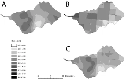
Fig. 4. Spatial distribution of total rainfall from March to October 2004 as derived by (A) ordinary kriging (mean value 492 mm), (B) operational available radar (mean value 490 mm) and (C) ordinary colocated cokriging (mean value 487 mm).

(7) var cckraing; spatially variable rainfall field, using ordi-nary colocated cokriging to make point predictions us-ing all the raus-ingauge stations of the experimental net-work as well as the operational KNMI radar data. (8) uni cckraing; same as scenario (7), but spatially

uni-form.

For the time series running from March to October 2004 there were 22 days (10%) with missing or incomplete radar images. No radar image means no scenario 5 until 8 for these days. In that case we used scenario 3 or 4 (ordinary kriging). Figure 3 shows the total rainfall amount for the period March to October 2004 for all 8 scenarios, that was calcu-lated by summing up the daily rainfall input of each model node. In Fig. 3 the spatially variable scenarios therefore show

a range of values whereas the spatially uniform scenarios only have a single value. The total rainfall amount of sta-tion Cabauw stands out as it is about 10% less than the other uniform rainfall fields. Nevertheless, this raingauge station is the only raingauge station of the automatic KNMI network located within the Lopikerwaard catchment and would have been a logical choice for hydrological studies.

date [dd−mm−yy]

average daily discharge [m3/min]

0 100 200 300

uni_cabauw

01−03−04 01−05−04 01−07−04 01−09−04

uni_bilt var_okraing

var_rarradar var_cckraing

0 100 200 300 uni_okraing

01−03−04 01−05−04 01−07−04 01−09−04 0

100 200 300

uni_rarradar uni_cckraing

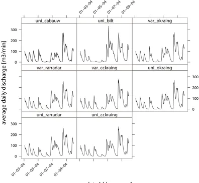
Fig. 5. Hydrographs of pumping station Koekoek for all the rainfall scenarios.

colocated cokriging and ordinary kriging, as could also be seen in Fig. 3. We also see in Fig. 4 that for the three spa-tially variable rainfall scenarios, the smallest amount of total rainfall fell in the mid-south and the largest amount of rain-fall fell in the west of the Lopikerwaard catchment.

4 Results

4.1 Discharge

With the hydrological model, we calculated for each rainfall scenario the average daily discharge of all the main pumping stations in the Lopikerwaard (Fig. 1d) for the period March to October 2004. We select two pumping stations, the one be-longing to the largest subcatchment (Koekoek) and the one belonging to the smallest subcatchment (Hoekse Molen), to show the hydrographs that result from the different rainfall scenarios. Figures 5 and 6 show the hydrographs for all

rain-fall scenarios of respectively pumping station Koekoek and Hoekse Molen. The hydrographs clearly show that for both pumping stations the rainfall scenario uni bilt deviates most from the other scenarios. This holds true for all 4 pump-ing stations. Two major differences in the hydrographs are caused by a rainfall event in the beginning of May that was registered in the Lopikerwaard but not in De Bilt and a rain-fall event in the beginning of July that was registered in De Bilt but was less prominent in the Lopikerwaard.

date [dd−mm−yy]

average daily discharge [m3/min]

0 10 20 30 40 50

uni_cabauw

01−03−04 01−05−04 01−07−04 01−09−04

uni_bilt var_okraing

var_rarradar var_cckraing

0 10 20 30 40 50

uni_okraing

01−03−04 01−05−04 01−07−04 01−09−04

0 10 20 30 40 50

uni_rarradar uni_cckraing

Fig. 6. Hydrographs of pumping station Hoekse Molen for all the rainfall scenarios.

Table 1. Percentage of days within March–October 2004 the discharge threshold value is exceeded. Threshold values vary per pumping station and are given underneath their names.

Scenario Hoekse Molen De Pleyt Keulevaart De Koekoek 15 m3/min 65 m3/min 65 m3/min 115 m3/min

uni cabauw 8 9 7 10

uni bilt 17 19 17 22

var okraing 15 17 11 17

uni okraing 13 15 10 16

var rarradar 16 17 12 15

uni rarradar 14 16 11 16

var cckraing 15 17 11 17

uni cckraing 12 14 11 16

pumping stations. Between the spatially variable and spa-tially uniform rainfall scenarios we see little difference in the discharge statistics.

standard deviation of the discharge. Table 1 shows the per-centage of days within the period March–October 2004 (212 days) that discharge threshold values were exceeded, with the threshold values given underneath the pumping stations. From this table we see again that for all subcatchments the rainfall scenario based on only data from station Cabauw (uni cabauw) leads to a lower amount of discharge peaks, while using data from only station De Bilt leads to a higher amount of discharge peaks in comparison to the other rainfall scenarios.

Although we cannot find structural differences in the time series statistics of discharge between spatially variable and spatially uniformed rainfall scenarios, there are certainly dif-ferences in discharge on specific days. These difdif-ferences are caused by the spatial distribution of rainfall.

4.2 Groundwater

For one randomly selected node, number 15552 located in the northwest, we show the development of groundwater level in time for all rainfall scenarios (Fig. 8). As we saw in the hydrographs, the development of groundwater level in time using rainfall scenario uni bilt differs most from the other rainfall scenarios. Again, the main differences are found around May and July. Using data only from station De Bilt results in lower groundwater levels in May and higher groundwater levels in July in comparison to the other scenar-ios.

We analyzed the development of groundwater level in time for all nodes. Figure 9 shows the spatial distribution of the mean temporal groundwater level and Fig. 10 shows the spa-tial distribution of the standard deviation of the temporal groundwater level. Note that the maps clearly show the in-print of the drainage network as a result of the artificially maintained water levels. To show the small differences be-tween the spatially uniform and spatially variable scenar-ios, the spatial distribution of the difference (variable mi-nus uniform scenarios) is shown as well. For all scenar-ios the spatial pattern of mean temporal groundwater level is more or less the same, although uni cabauw and uni bilt both show slightly lower groundwater levels in the eastern part of the Lopikerwaard. Using spatially variable instead of spatially uniform rainfall scenarios leads to slightly (2 cm) higher mean groundwater levels in the west and east and slightly (2 cm) lower groundwater levels in the middle part of the Lopikerwaard if we use information from the raingauges. Using information from the radar leads to slightly (2 cm) lower groundwater levels in the west and slightly higher (2– 4 cm) groundwater levels in the eastern part of the Lopiker-waard. The spatial pattern of the standard deviation of the temporal groundwater level of uni bilt differs most from the other scenarios, showing an overestimation of the temporal variation of groundwater level. Uni cabauw leads to slightly lower standard deviations. Using spatially distributed rain-fall scenarios instead of spatially uniform scenarios leads to

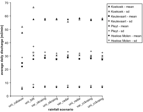
0 10 20 30 40 50 60 70 rainfall scenario av er ag e da ily d is ch ar ge [m 3/ m in ]

Koekoek - mean Koekoek - sd Keulevaart - mean Keulevaart - sd Pleyt - mean Pleyt - sd Hoekse Molen - mean Hoekse Molen - sd

uni_cabauw var_ok

raing uni_bilt uni_ok raing uni_radar uni_cck raing

var_radar _{var_cck}raing

Fig. 7. Mean and standard deviation of the average daily dis-charge for all 4 pumping stations in the Lopikerwaard for the period March–October 2004.

higher standard deviations in the north and lower standard deviation in the south.

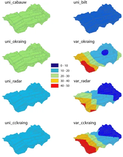
To get an impression of the effect of the different rainfall scenarios on day-to-day spatial variability, we selected one day with highly spatially variable rainfall. Figure 11 shows the rainfall within the Lopikerwaard for all rainfall scenarios at 1 May 2004. Figure 12 shows its effect on the ground-water level (m from ground level) throughout the Lopiker-waard for all the rainfall scenarios. Again, rainfall scenario uni bilt differs most from the other rainfall scenarios. At 1 May 2004 we see that the groundwater level within the Lopikerwaard using rainfall scenario uni bilt is much lower than if we use rainfall information from the catchment itself, even if we use only one raingauge (uni cabauw). The spa-tially variable rainfall scenarios all show a different spatial pattern of groundwater level than the corresponding spatially uniform rainfall scenarios. Using spatially variable rainfall scenarios leads at 1 May 2004 to deeper groundwater levels in the north-eastern part of the Lopikerwaard.

4.3 Soil moisture

date [dd−mm−yy]

groundwaterlevel [m beneath ground level]

−0.8 −0.6 −0.4 −0.2

uni_cabauw

01−03−04 01−05−04 01−07−04 01−09−04

uni_bilt uni_okraing

uni_rarradar uni_cckraing

−0.8 −0.6 −0.4 −0.2

var_okraing

01−03−04 01−05−04 01−07−04 01−09−04 −0.8

−0.6 −0.4 −0.2

var_rarradar var_cckraing

Fig. 8. Development of groundwater level [m from ground level] in time of node number 15552 for all rainfall scenarios. The location of node number 15552 is given in lower right corner.

Also for soil moisture we analyzed its development in time for all nodes. The results are similar to that of groundwater and not shown here. The spatial pattern of the mean temporal soil moisture content is for all the rainfall scenarios more or less the same. The temporal variance in soil moisture content is overestimated when using rainfall information from station De Bilt in comparison to the other rainfall scenarios. For the other scenarios, the spatial pattern of temporal variation of soil moisture content is more or less the same.

To get insight in the day-to-day variability of soil mois-ture, Fig. 14 shows the effect of the 1 May rainfall event (Fig. 11) on the soil moisture content within the Lopiker-waard. The soil within the Lopikerwaard using rainfall sce-nario uni bilt is much drier than if we use rainfall informa-tion from the catchment itself, even if we use only one rain-gauge (uni cabauw). The spatially variable rainfall scenar-ios all show a different spatial pattern of soil moisture than

the corresponding spatially uniform rainfall scenarios. Us-ing spatially variable rainfall scenarios leads at 1 May 2004 to higher soil moisture content in the western part and lower soil moisture content in the north-eastern part of the Lopik-erwaard. This corresponds with the spatial pattern of rainfall (Fig. 11). For all scenarios, the lowest soil moisture con-tents correspond with the urban areas of the Lopikerwaard (Fig. 1b).

5 Conclusions and discussion

< -1.0

-1.0 - -0.7

-0.7 - -0.6

-0.6 - -0.5

-0.5 - -0.4

-0.4 - -0.3

-0.3 - -0.2

-0.2 - -0.1

-0.1 - 0

> 0

< -1.0

-1.0 - -0.7

-0.7 - -0.6

-0.6 - -0.5

-0.5 - -0.4

-0.4 - -0.3

-0.3 - -0.2

-0.2 - -0.1

-0.1 - 0

> 0

mean groundwater level [m from ground level]

uni_cabauw

uni_bilt

uni_cckraing

uni_radar

uni_okraing

var_cckraing

var_radar

var_okraing

difference var and uni scenarios

uni_cabauw

uni_bilt

uni_cckraing

uni_radar

uni_okraing

var_cckraing

var_radar

0.00 - 0.05 0.05 - 0.10 0.10 - 0.15 0.15 - 0.20 > 0.20

standard deviation groundwater level [m] difference var and uni scenarios

var_okraing

uni_cabauw

uni_bilt

uni_okraing

var_okraing

uni_radar

var_radar

uni_cckraing

var_cckraing

0 - 10 10 - 20 20 - 30 30 - 40 40 - 50

Fig. 11. Spatial pattern of rainfall in mm on 1 May 2004 for the different rainfall scenarios in the Lopikerwaard.

great risk in using a single raingauge, especially when lo-cated outside the catchment, for the prediction of discharge, spatial distribution of soil moisture and spatial distribution of groundwater level. For the general hydrological behaviour, this study corroborates the conclusion stated by Obled et al. (1994) that the spatial distribution of rainfall must be taken into account more because it improves the basaverage

in-coming volume rather than because of some dynamic inter-actions with flow-generating processes. However, for par-ticular days, incorporating spatially variable information on rainfall is of great importance for the spatial distribution of interior catchment response.

uni_radar

var_radar

uni_cckraing

var_cckraing

uni_okraing

uni_cabauw

uni_bilt

var_okraing

< -1.0

-1.0 - -0.7

-0.7 - -0.6

-0.6 - -0.5

-0.5 - -0.4

-0.4 - -0.3

-0.3 - -0.2

-0.2 - -0.1

-0.1 - 0

> 0

Fig. 12. Spatial variation of groundwater level [m from ground level] on 1 May 2004 for the different rainfall scenarios.

amount of rainfall for the period March–October 2004 as estimated by the operational radar corresponds to the total amount found by the kriged rainfall fields based on 30 rain-gauges within the catchment. The spatial variation (range of values) of the total rainfall was found to be higher for radar than for the kriged raingauges. This is, among other factors influencing radar-estimated rainfall accuracy, maybe

date [dd−mm−yy]

relative soil moisture

0.42 0.44 0.46 0.48 0.50 0.52

uni_cabauw

01−03−04 01−05−04 01−07−04 01−09−04

uni_bilt uni_okraing

uni_radar uni_cckraing

0.42 0.44 0.46 0.48 0.50 0.52

var_okraing

01−03−04 01−05−04 01−07−04 01−09−04 0.42

0.44 0.46 0.48 0.50 0.52

var_radar var_cckraing

Fig. 13. Development of soil moisture content in time of node number 15552 for all rainfall scenarios. The location of node 15552 is given in lower right corner.

can conclude that using radar-estimated rainfall input leads to similar (or slightly more varying) discharges as using a dense network of raingauges. This shows that standard range-corrected radar products are sufficiently informative about the spatial variability of rainfall to be used in hydrological applications.

This study uses a hydrological model to study the sensi-tivity of spatially variable rainfall on interior catchment sponse. This can of course only be done if the model re-flects the true catchment response. As often mentioned for this kind of studies, the results are dependent on the spatio-temporal variation of rainfall and the characteristics of the catchment, or in this case the characteristics of the hydrolog-ical model. It is known that there is a space-time correlation in rainfall variability. Krajewski et al. (1991) found that basin response shows higher sensitivity with respect to the tempo-ral resolution than to spatial resolution of the rainfall data.

This study shows that even for daily rainfall it is important to take account of the spatial rainfall variability, if one aims to predict the internal hydrological state of the catchment.

uni_cabauw

uni_bilt

uni_okraing

var_okraing

uni_radar

var_radar

uni_cckraing

var_cckraing

0.00 - 0.20

0.20 - 0.30

0.30 - 0.35

0.35 - 0.40

0.40 - 0.45

0.45 - 0.50

0.50 - 0.60

0.60 - 0.70

Fig. 14. Spatial pattern of soil moisture content [–] on 1 May 2004 for the different rainfall scenarios in the Lopikerwaard.

the potential and necessity of using the operational available radar products in hydrological studies.

Acknowledgements. J. M. Schuurmans was financially supported

by TNO.

Edited by: J. D. Kalma

References

Arnaud, P., Bouvier, C., Cisner, L., and Dominguez, R.: Influence of rainfall spatial variability on flood prediction, J. Hydrol., 260, 216–230, 2002.

Battan, L. J.: Radar Observations of the Atmosphere, University of Chicago Press, Chicago, 1973.

models to rainfall data at different spatial scales, Hydrol. Earth Syst. Sci., 4, 653–667, 2000,

http://www.hydrol-earth-syst-sci.net/4/653/2000/.

Carpenter, T. M., Georgakakos, K. P., and Sperfslagea, J. A.: On the parametric and NEXRAD-radar sensitivities of a distributed hydrological model suitable for operational use, J. Hydrol., 253, 169–193, 2001.

Cressie, N. A. C.: Statistics for spatial data, Revised Edition, John Wiley & Sons, Inc., New York, 1993.

De Bruin, H. A. R.: From Penman to Makkink, in: Proc. and Inf. Vol. 39, TNO Committee on Hydrological Research, pp. 5–31, 1987.

Gekat, F., Meischner, P., Friedrich, K., Hagen, M., Koistinen, J., Michelson, D. B., and Huuskonen, A.: Weather Radar, Princi-ples and Advanced Applications. Springer, Berlin, Germany, Ch. The State of Weather Radar Operations, Networks and Products, 2004.

Goodrich, D. C., Faures, J. M., Woolhiser, D. A., Lane, L. J., and Sorooshian, S.: Measurements and analysis of small-scale con-vective storm rainfall variability, J. Hydrol., 173, 283–308, 1995. Goovaerts, P.: Geostatistics for Natural Resources Evaluation,

Ox-ford University Press, New York, 1997.

Holleman, E. T., Zaadnoordijk, W. J., Meuter, N. H., Roe-landse, A. S., and Veldhuizen, A.: Wateropgave HDSR-West (in Dutch), Tech. Rep. Reference: 9M8931/R00002/HTD/Rott1, Royal Haskoning, 2005.

Holleman, I.: VPR adjustment using a dual CAPPI technique, in: Proc. of ERAD, Vol. 2, Copernicus GmbH, pp. 25–30, 2004. Isaaks, E. H. and Srivastava, R. M.: Applied Geostatistics, Oxford

University Press, New York, 1989.

Krajewski, W. F., Lakshmi, V., Georgakakos, K., and Jain, S.: A monte carlo study of rainfall sampling effect on a distributed catchment model, Water Resour. Res., 27(1), 119–128, 1991.

Krajewski, W. F. and Smith, J. A.: Radar hydrology: rainfall esti-mation, Adv. Water Resour., 25(8–12), 1387–1394, 2002. Obled, C., Wending, J., and Beven, K.: The sensitivity of

hydro-logical models to spatial rainfall patterns: an evaluation using observed data, J. Hydrol., 159, 305–333, 1994.

O’Connell, P. E. and Todini, E.: Modelling of rainfall, flow and mass transport in hydrological systems: an overview, J. Hydrol., 175, 3–16, 1996.

Querner, E. P.: Description and application of the combined surface and groundwater flow model MOGROW, J. Hydrol., 192, 158– 188, 1997.

Schuurmans, J. M., Bierkens, M. F. P., Pebesma, E. J., and Uijlen-hoet, R.: Automatic prediction of high-resolution daily rainfall fields for multiple extents: the potential of operational radar, J. Hydrometeorol., accepted, 2007.

Shah, S. M. S., O’Connel, P. E., and Hosking, J. R. M.: Modelling the effects of spatial variability in rainfall on catchment response. 2. experiments with distributed and lumped models, J. Hydrol., 175, 89–111, 1991.

Wessels, H. R. A. and Beekhuis, J. H.: Stepwise procedure for sup-pression of anomalous ground clutter, in: COST-75 Seminar on Advanced Radar Systems, EUR 16013 EN, pp. 270–277, 1997. Winter, T. C., Rosenberry, D. O., and Sturrock, A. M.: Evaluation

of 11 equations for determining evaporation for a small lake in the North Central United States, Water Resour. Res., 31(4), 983– 993, 1995.