Global isoscapes for δ18O and δ2H in precipitation: improved prediction using regionalized climatic regression models

Hydrol. Earth Syst. Sci., 17, 4713–4728, 2013 www.hydrol-earth-syst-sci.net/17/4713/2013/ doi:10.5194/hess-17-4713-2013

© Author(s) 2013. CC Attribution 3.0 License.

Hydrology and

Earth System

Sciences

Global isoscapes for

δ

18

O and

δ

2

H in precipitation: improved

prediction using regionalized climatic regression models

S. Terzer, L. I. Wassenaar, L. J. Araguás-Araguás, and P. K. Aggarwal

International Atomic Energy Agency, Isotope Hydrology Section, Vienna International Centre, Vienna, 1400, Austria Correspondence to: S. Terzer ([email protected])

Received: 23 April 2013 – Published in Hydrol. Earth Syst. Sci. Discuss.: 11 June 2013 Revised: 8 October 2013 – Accepted: 24 October 2013 – Published: 29 November 2013

Abstract. A regionalized cluster-based water isotope

predic-tion (RCWIP) approach, based on the Global Network of Isotopes in Precipitation (GNIP), was demonstrated for the purposes of predicting point- and large-scale spatio-temporal patterns of the stable isotope composition (δ2H, δ18O) of precipitation around the world. Unlike earlier global do-main and fixed regressor models, RCWIP predefined 36 cli-matic cluster domains and tested all model combinations from an array of climatic and spatial regressor variables to obtain the best predictive approach to each cluster domain, as indicated by root-mean-squared error (RMSE) and var-iogram analysis. Fuzzy membership fractions were there-after used as the weights to seamlessly amalgamate results of the optimized climatic zone prediction models into a sin-gle predictive mapping product, such as global or regional amount-weighted mean annual, mean monthly, or growing-seasonδ18O/δ2H in precipitation. Comparative tests revealed the RCWIP approach outperformed classical global-fixed regression–interpolation-based models more than 67 % of the time, and clearly improved upon predictive accuracy and precision. All RCWIP isotope mapping products are available as gridded GeoTIFF files from the IAEA website (www.iaea.org/water) and are for use in hydrology, climatol-ogy, food authenticity, ecolclimatol-ogy, and forensics.

1 Introduction

Spatial patterns in stable hydrogen and oxygen isotope ra-tios of precipitation were first observed in the 1950s (Epstein and Mayeda, 1953; Friedman, 1953; Dansgaard, 1954; Craig, 1961), and increasingly revealed as long-termδ2H andδ18O data sets from around the world accumulated in the

Interna-tional Atomic Energy Agency’s (IAEA) global network of isotopes in precipitation (GNIP – Fig. 1) (Dansgaard, 1964; Rozanski et al., 1993; Aggarwal et al., 2010; IAEA/WMO, 2013). The strong covariance ofδ2H and δ18O in precipi-tation (Craig, 1961) supported the construction of local and regional isotopic “meteoric water lines”, which provided the basis, for example, upon which to assess the origin of mod-ern and ancient ground water (Rozanski, 1985; Clark and Fritz, 1997) and its interaction with surface water resources (Kendall and McDonnell, 1998; Froehlich et al., 2005).

4714 S. Terzer et al.: Global isoscapes forδ18O andδ2H in precipitation

Discussion

P

ap

er

|

Discussion

P

ap

er

|

Dis

cussion

P

ap

er

|

Discussion

P

ap

er

|

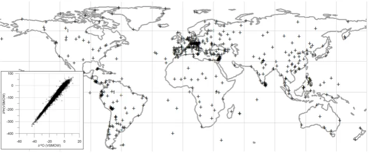
Fig. 1.

Global map of GNIP stations used for RCWIP modelling. All stations represented 2 to 52 yr of

monthly

δ

O or

δ

H and climate data from 1960 to 2009. Inset: a cross-plot of

δ

O versus

δ

H at

stations used, yielding a GMWL of

δ

_{H = 7.91}

_δ

_{O + 8.72 (}

_R

_{= 0}

_.

₉₇₆

_,

_n

_{= 576}

_).

figure

30

Fig. 1. Global map of GNIP stations used for RCWIP modeling. All stations represented 2 to 52 yr of monthlyδ18O orδ2H and climate

data from 1960 to 2009. Inset: a cross-plot ofδ18O versusδ2H at stations used, yielding a GMWL ofδ2H = 7.91δ18O + 8.72 (R2=0.976,

n=576).

driven by and premised upon the foundational global patterns ofδ2H andδ18O in precipitation, were required.

Early attempts at producing maps ofδ2H orδ18O patterns in precipitation (Sheppard et al., 1969; Yurtsever and Gat, 1981) were later improved with geographical information systems (GIS) and the online availability of spatially exten-sive water isotope (GNIP) and climatic data sets (Rozanski et al., 1993; Dutton et al., 2005; Welker, 2012). Descriptive spatial maps ofδ2H orδ18O in precipitation were first made using simple inverse distance-weighted approaches (Birks et al., 2002; Aggarwal et al., 2010). Thereafter, more com-plex multiple regression and interpolation prediction mod-els were widely used (Bowen and Wilkinson, 2002; Bowen and Revenaugh, 2003). In particular, the approach of Bowen and Wilkinson – hereafter called model M1 – used fixed predictor variables (absolute latitude, squared latitude, alti-tude) to obtain the response variable (δ2H/δ18O in precipita-tion) and an interpolation parameter to optimize the fitting model. Because isotope ratios show a strong linear corlation with mean annual air temperature in nontropical re-gions, model M1 was able to explain 58–61 % of the iso-topic variance in precipitation over a globally gridded do-main. Model M1 did not downscale well particularly into tropical parts of the world, resulting in poorer fits between isotope data and model results (e.g., Africa, Asia, etc.). Some researchers therefore constrained the geographical domain (Liu et al., 2008) or added meteorological explanatory re-gressor variables at a global scale (van der Veer et al., 2009; Bowen, 2010). Others combined meteorological (e.g., sur-face air temperature, relative humidity, snowfall amount, etc.) and geospatial variables in order to obtain improved re-gressions/interpolations of precipitation isotope composition for specific regions such as Austria (Liebminger et al., 2006), the eastern Mediterranean (Lykoudis and Argiriou, 2007), and Canada (Delavau et al., 2011). In a different approach, a spatially dense groundwater isotope network was used as a

“proxy” for mean annual precipitation and used generalized linear models (GLMs) and multiple predictor variables (ele-vation, precipitation amount, latitude, basin, and their inter-actions) to explain 81 % of the isotopic variance and patterns in precipitation in Mexico (Wassenaar et al., 2009). All of the above regionalized multivariate regression and interpo-lation approaches resulted in markedly improved predictive outcomes across some regions as manifested by (1) higher coefficients of determinations (R2) between the measured and modeled data and (2) lower predictive uncertainties or residuals when compared to model M1 (a summary of mod-els is given in Table 1). However, because regional modmod-els were arbitrarily fitted to small geographical domains, they were not applicable at the global scale.

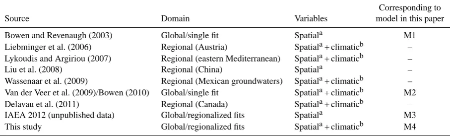
Table 1. Examples of global and regional water isotope models and type of predictive spatial and climatic variables used for the isotopic

composition of precipitation and ground water.

Corresponding to

Source Domain Variables model in this paper

Bowen and Revenaugh (2003) Global/single fit Spatiala M1

Liebminger et al. (2006) Regional (Austria) Spatiala+ climaticb –

Lykoudis and Argiriou (2007) Regional (eastern Mediterranean) Spatiala+ climaticb –

Liu et al. (2008) Regional (China) Spatiala –

Wassenaar et al. (2009) Regional (Mexican groundwaters) Spatiala+ climaticb –

Van der Veer et al. (2009)/Bowen (2010) Global/single fit Spatiala+ climaticb M2

Delavau et al. (2011) Regional (Canada) Spatiala+ climaticb –

IAEA 2012 (unpublished data) Global/regionalized fits Spatiala M3

This study Global/regionalized fits Spatiala+ climaticb M4

a_{Spatial variables shall be defined as any combination of the following: latitude, longitude, and elevation (including derived parameters like squared or absolute}

latitude).bclimatic variables are defined as any combination of the following: precipitation amount, air temperature, vapor pressure and other climate-related

variables (wind speed, snow amount, relative humidity, precipitable water/moisture residence time, etc.).

uncertainty of precipitation isoscapes were used to illustrate improved RCWIP outcomes.

2 Materials and methods

RCWIP employed the well-established linear prediction model based on multiple regressions of station-based precipi-tation isotope and climatic data and the interpolation of resid-uals (Bowen and Revenaugh, 2003). RCWIP differed from this key earlier work in that it used the best performing model from a suite of regionalized domain multivariate regression equations to determine the isotopic composition of precipita-tion at a known locaprecipita-tionias a function of the selected pre-dictor variables available. A comparison between model M1 and the RCWIP approach is described in Fig. 2. To accom-modate regionalization, RCWIP introduced additional steps of formation of subsets of station-based data as well as the gridded data sets according to their climatic clustering prop-erties, as well as the determination of model parameter set-tings and the coefficient estimations for each climatic cluster, as described in turn below.

2.1 δ2H andδ18O isotope and spatial data

The precipitation stable isotope data set used was comprised of monthly composites ofδ2H andδ18O in precipitation from worldwide stations archived in the GNIP database (Aggar-wal et al., 2010), supplemented by compatible monthly iso-tope data from published papers (Wang and Peng, 2001; Kra-lik et al., 2003; Kurita and Ichiyanagi, 2008). The tempo-ral span of isotopic data records was constrained to 1960– 2009, although fewer than 100 stations were fully contem-poraneous over this time frame. The longest serving GNIP stations spanned 20–52 yr of isotopic records. Additionally, stations that did not have over two years of monthly iso-topic records were omitted to avoid seasonal biases

aris-Discussion

P

ap

er

|

Discussion

P

ap

er

|

Dis

cussion

P

ap

er

|

Discussion

P

ap

er

|

Fig. 2.Workflow of the regression-interpolation models for predicting the isotopic composition of

pre-cipitation around the globe. The upper panel(a)shows the workflow of the fixed regressor, global domain

Model M1 (Bowen and Wilkinson, 2003). The lower panel(b)shows the workflow of RCWIP with the

addition of climate data, regionalization and the use of flexible regressors (Models M2–M4). 31

Fig. 2. Workflow of the regression–interpolation models for

predict-ing the isotopic composition of precipitation around the globe. The upper panel (a) shows the workflow of the fixed regressor, global domain model M1 (Bowen and Wilkinson, 2002). The lower panel

(b) shows the workflow of RCWIP with the addition of climate data,

regionalization, and the use of flexible regressors (models M2–M4).

4716 S. Terzer et al.: Global isoscapes forδ18O andδ2H in precipitation

obtained from the GNIP database or from digital elevation models.

The stable isotope data in the GNIP database were com-posed of station-based point measurements with substantial gaps in spatio-temporal coverage (Rozanski et al., 1993; Ag-garwal et al., 2010). Concerns surrounding the pooling and use of noncontiguous data sets for spatial isotope mapping have previously been discussed (Bowen, 2010). Furthermore, nearly half of the longest-serving GNIP stations showed time trends when adjusted for seasonality, although there was no obvious process to explain the trends. Additionally, for trend-ing stations, the mean interannual rate of isotopic change was rather small (δ18O<0.03 ‰ per year) in comparison to sea-sonal isotopic fluctuations, historical measurement error, and methodological changes, but the cumulative decadal change appeared significant over longer time frames for a few re-gions (Table S1 in the Supplement). For this paper, we ac-cepted the spatio-temporal limitations of the GNIP data set in pooling noncontiguous decadal-scale data sets (Bowen, 2010). However, users of isoscape mapping efforts must re-main alert to inherent assumption of temporal constancy in the isoscape maps, particularly when the studies may be sen-sitive to interannual or stochastic variability (e.g., plant or food traceability studies).

2.2 Climate data

Climatological variables (monthly precipitation amount, air temperature, vapor pressure) corresponding to the iso-tope sampling stations were also obtained from the GNIP database. When corresponding meteorological data were un-available, averaged climate data (monthly, annual) was ob-tained from the nearest station in the Global Historical Cli-mate Network station (GHCN) (Peterson et al., 1998). If a nearby GHCN station was not available, climatic parame-ters were obtained from the CRU-CL 2.1 data set (New et al., 2002). The precipitation amount data were natural-log-transformed to achieve normality and to linearize the rela-tionship withδ2H and δ18O. Point-based data on monthly mean precipitable water was included into the array of cli-matic variables as it helped define the mean residence time of vapor, which had high predictive power for the isotopic composition of precipitation in tropical regions (Aggarwal et al., 2012).

Gridded data sets of spatial and climatic variables (mean monthly/annual temperature, precipitation, and relative hu-midity) were extracted from the CRU-CL 2.1 data set (New et al., 2002) at a resolution of 10 arcmin. Vapor pressure was calculated from temperature and relative humidity us-ing the equations given by the World Meteorological Organi-zation (WMO, 2008). Gridded precipitable water data were obtained by interpolation of point-based information; how-ever, the use of remotely sensed data (e.g., NASA EOS At-mospheric Infrared Sounder) is anticipated in the future.

2.3 Climatic zone clustering

Because climatic parameters are spatially continuous, sharply drawn climatic classification boundaries on a map pose an unrealistic depiction of their spatially continuous dis-tribution (McBratney and Moore, 1985). Climatic classes, however, may be useful in varied forms (e.g., plant hardi-ness zones). To avoid sharp boundary domain constraints, fuzzy clustering techniques, including fuzzyc-means (FCM; Bezdek, 1981; Cannon et al., 1986), were used to (1) sta-tistically reduce the global climatic data set to a number of manageable and unique spatial domain clusters and (2) to seamlessly overlap the determined climatic class boundaries. Fuzzy clusters used fractional membership values (e.g., a GNIP station may be 60 % in cluster A and 40 % in cluster B) rather than a strict binary criterion (whether it belongs or not) to classify stations or points on the landscape. To achieve this, the FCM routine randomly seeded cluster centroids in the data space and iteratively adjusted their positions to min-imize the total of all distances between the input data points and the centroids until a convergence criterion (such as min-imal improvement from one iteration to the next, or preset number of iterations) was reached. Cannon et al. (1986) de-fined the fuzzyc-means function by

Jm(U, ϑ )= n

X

k=1

c

X

i=1

(uik)m(dik)2, (1)

with U being the fuzzy membership matrix for a set of cen-troidsϑ=(ϑ1, ϑ2, . . ., ϑc). The distancedik between thekth

data pointxk and theith centroidϑi was calculated as

d_ik2 = kxk−ϑik2. (2)

m∈_[1,∞_{] was a fuzzification (i.e., smoothing) factor that} indicated the sharpness of transition between two fuzzy clus-ters, withm=1 indicating a crisp boundary line. Cannon et al. (1986) reported a value of 1.1< m <5 as “useful”. For RCWIP clustering, a factor ofm=1.5 was experimentally determined as a suitable compromise between fuzzy bound-aries and spatial explicitness: while a smoothing factor of 1.0 would have resulted in line boundaries (no fuzzy transitions), we experimented extensively with the smoothing factor and found out thatm >1.5 would have led to inordinately large clusters extending, for example, from one continent into an-other ignoring the ocean in between. Since our approach was focused on land areas, we empirically found that m=1.5 was a suitable (albeit arbitrary) compromise to balance be-tween terrestrially meaningful clusters and obtaining smooth transitions between them.

S. Terzer et al.: Global isoscapes forδ18O andδ2H in precipitation 4717

P

ap

er

|

Discussion

P

ap

er

|

Dis

cussion

P

ap

er

|

Discussion

P

ap

er

|

Fig. 3.

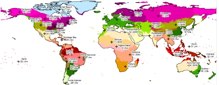
Map of 36 climatic zone domains used in RCWIP, derived by fuzzy clustering but here shown

with defined boundaries. The “+” symbol denotes the spatial location of each climatic zone centroid.

The descriptions of each of these climatic zones are denoted by a number (Zone #) and a K¨oppen-Geiger

climatic zone description (e.g. Dfc). These are fully tabulated in Table 2 and Sheet S2 in the Supplement.

32

Fig. 3. Map of 36 climatic zone domains used in RCWIP, derived by fuzzy clustering but here shown with defined boundaries. The “+”

symbol denotes the spatial location of each climatic zone centroid. The descriptions of each of these climatic zones are denoted by a number (zone no.) and a Köppen–Geiger climatic zone description (e.g., Dfc). These are fully tabulated in Table 2 and Sheet S2 in the Supplement.

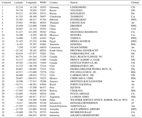
of climatic input variables, although it was generally recom-mended that the number of clusters be twice the number of input variables (McBratney and Moore, 1985). Our reason-ing was practical and by trial and error, because we found using more climatic clusters led to difficulties in subdivid-ing the unevenly distributed GNIP data set (Fig. 1). Each GHCN data point was then assigned a weight based on its proximity to its nearby stations, whereby a GHCN station’s average distance to its five closest neighbors was normal-ized to this parameter’s average over the whole GHCN data set. Globally, the GHCN data were heavily overrepresented in some regions, and unconstrained FCM clustering would have resulted in an excessive number of climatic clusters in weather-data-rich countries like the USA, Canada, Australia, and China (Table 2). This exercise resulted in the identifica-tion of 36 climatic clusters.

The 36 FCM-derived climatic clusters were then subjected to a first-order evaluation of their appropriateness by compar-ing their features to the well-known Köppen–Geiger climate classification scheme (Kottek et al., 2006). Our evaluation also consisted of determining whether each FCM-defined cli-mate zone cluster was consistent with the geographical lo-cation of the cluster centroid. Following this, some offline manual adjustments were needed. These changes mainly in-volved manually moving the geographic location of FCM de-rived climatic centroid to the closest station of the WMO’s Global Surface Network (GSN). In a few cases (e.g., Antarc-tica), cluster centroids were moved to entirely new positions to better cover those areas that were underrepresented by the automated FCM clustering. A spreadsheet of the FCM out-puts, as well as the geographical positions and climate data averages of the 36 centroids along with descriptions of each climatic zone was tabulated in the supplementary material (Table S2).

The final positioning of the 36 global climatic zone cen-troids served as the fundamental basis for defining the RCWIP subsets, and was applied to the GNIP station data

set as well as the gridded climatic data sets, resulting in each GNIP station or each CRU grid cell being assigned a fuzzy cluster membershipuik:

uik=

1

d2_ik

(m−1)−1

c

P

i=1

1

d_ik2

(m−1)−1. (3)

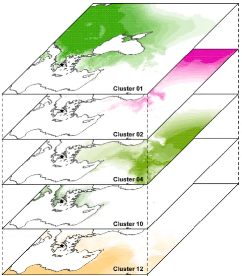
Membership fractions of <0.02 were considered insignifi-cant and omitted in order to give more weight to the main membership fractions of a data point or grid cell. The re-maining fractions were renormalized to their sums. Fuzzy membership fractions were also used to layer-stack the mem-bership of the GNIP stations to each climatic zone. The cri-terion used for including a GNIP station in a given climatic zone regression subset was a minimum membership fraction of 0.1. A map of the 36 climatic cluster zones used is shown in Fig. 3. Figure 4 also provides an illustrative example of the spatial depiction of clustering membership fractions and the amalgamation for a selected geographical region.

This clustering procedure also provided a useful exercise for categorization of the GNIP stations, since it afforded a statistically robust and unbiased (e.g., by arbitrary bound-aries) means to group subsets of “climatically similar” GNIP stations. One benefit of this analysis is that it allowed a visu-alization of climatically similar zones around the Earth that were (1) overrepresented by current and historical GNIP data collections (e.g., Europe), (2) lacking in GNIP data to be targeted for future stations, and (3) historically underrepre-sented (e.g., compare the GNIP station distribution in Fig. 1 with zones in Fig. 3).

2.4 Regression models

4718 S. Terzer et al.: Global isoscapes forδ18O andδ2H in precipitation

Table 2. The ID number, geographic centroid location, climatic zone, and WMO station of the climatic clusters used in RCWIP.

Centroid Latitude Longitude WMO Country Station Climate

1 52.210 14.120 10393 Germany LINDENBERG Cfb

2 59.318 39.926 27037 Russia VOLOGDA Dfb

3 58.317 82.950 29231 Russia KOLPASEVO Dfc

4 41.333 69.300 38457 Uzbekistan TASHKENT Csa

5 25.383 68.417 41764 Pakistan HYDERABAD BWh

6 19.961 99.881 48303 Thailand CHIANG RAI Aw

7 43.650 112.000 53068 China ERENHOT BWk

8 29.667 91.133 55591 China LHASA Cwb

9 31.417 121.450 58362 China SHANGHAI (BAOSHAN) Cfa

10 34.300 −6.595 60120 Morocco KENITRA Csa

11 14.900 5.250 61043 Niger TAHOUA BWh

12 31.325 27.222 62306 Egypt MERSA MATRUH BWh

13 −6.167 35.767 63862 Tanzania DODOMA BSh

14 7.350 13.567 64870 Cameroon NGAOUNDERE Aw

15 −25.742 28.183 68262 South Africa PRETORIA EENDRACHT Cwa

16 64.816 −147.877 70261 USA FAIRBANKS/INT., AK Dfc

17 68.776 −81.244 71320 Canada HALL BEACH CLIMATE, NU ET

18 53.217 −105.667 71869 Canada PRINCE ALBERT A, SASK Dfb

19 49.383 −126.545 71894 Canada ESTEVAN POINT CS, BC Cfb

20 32.333 −88.750 72234 USA MERIDIAN/KEY, MS. Cfa

21 40.667 −89.683 72532 USA PEORIA/GREATER PEORIA MUN., IL. Dfa

22 42.917 −112.600 72578 USA POCATELLO/MUN., ID. BSk

23 46.868 −68.014 72712 USA CARIBOU/MUN., ME. Dfb

24 28.667 −106.033 76225 Mexico CHIHUAHUA, CHIH. BSh

25 18.500 −77.917 78388 Jamaica MONTEGO BAY/SANGSTER Aw

26 −10.717 −48.583 83064 Brazil PORTO NACIONAL Aw

27 −3.783 −73.300 84377 Peru IQUITOS Af

28 −17.583 −69.600 85230 Bolivia CHARANA BSk

29 −53.005 −70.839 85934 Chile PUNTA ARENAS Cfc

30 −29.383 −66.817 87217 Argentina LA RIOJA AERO. BSh

31 7.340 134.489 91408 Palau WEATHER SERVICE OFFICE, KOROR, PALAU WCI. Af

32 −9.417 160.050 91520 Solomon Is. HONIARA/HENDERSON Af

33 −17.555 −149.614 91938 French Polynesia TAHITI-FAAA Am

34 −23.795 133.889 94326 Australia ALICE SPRINGS AIRPORT BWh

35 −33.600 150.776 95753 Australia RICHMOND RAAF Cfa

36 −6.183 106.833 96745 Indonesia JAKARTA/OBSERVATORY Am

fixed regressor variables, as described previously (Bowen and Wilkinson, 2002; Bowen and Revenaugh, 2003). Model M1 therefore served as the basis upon which to assess RCWIP performance. Model M2 comprised the same global domain model of M1, but used a covariate best fit instead of a fixed regressor combination. To further accommodate regionalization through the use of the climatic clustering, model M3 used the same approach as M1, but using fixed regressors for each of the 36 individual climatic clusters. The most flexible model of all – model M4 – used all 36 region-alized climatic clusters and used the best fit of all regressor variable combinations for each zone. A process flowchart for RCWIP regression modeling is shown in Fig. 5.

Climatically regionalized best-fit flexible regression mod-els were derived from all possible combinations of the fol-lowing variables: latitude, longitude, elevation, air tempera-ture, precipitation amount, vapor pressure, and precipitable water. Any of the 120 combinations of these explanatory re-gressors were tested and ranked according to their coefficient

of determination (R2). For models M2 and M4, the best-fit combinations were selected if they met an acceptance crite-rion ofR2 of ≥0.5, and the number of remaining degrees of freedom was≥7.5 times the number of independent vari-ables (for M2, this was always the case). For model M4, this procedure was performed on all 36 climatic clusters; how-ever, if no suitable regression equation satisfying the accep-tance criteria was obtained for a given cluster or month, the global domain best-fit regression equation (M2) for the corre-sponding month was applied by default to the cluster/month. Since M2 was effectively a “backup solution” for preferred M4 model, it was not discussed further.

The “fixed-regressor” models M1 and M3 were applied to the same climatic clustering, but their equations were derived on the general form given by Eq. (4):

δ18O=alat2+b|lat| +c (alt)+d, (4)

whereδ18O (or δ2H) was the predicted value; a, b, andc

S. Terzer et al.: Global isoscapes forδ18O andδ2H in precipitation 4719

Discussion

P

ap

er

|

Discussion

P

ap

er

|

Dis

cussion

P

ap

er

|

Discussion

P

ap

er

|

Fig. 4.

Example of fuzzy climatic zone layering and amalgamation for a geographical domain around

the Mediterranean- Black Sea region. The five climatic clusters in this spatial domain (Climatic clusters

1, 2, 4, 10 and 12) were overlain, with degree of color saturation of each indicative of the fractional

membership for each grid cell. The GNIP station in Athens (indicated by a small star sign), Greece, for

example, holds membership fractions of 0.14, 0.34 and 0.52 in clusters 1, 10 and 12, respectively.

33

Fig. 4. Example of fuzzy climatic zone layering and amalgamation

for a geographical domain around the Mediterranean–Black Sea re-gion. The five climatic clusters in this spatial domain (climatic clus-ters 1, 2, 4, 10, and 12) were overlain, with degree of color satura-tion of each indicative of the fracsatura-tional membership for each grid cell. The GNIP station in Athens (indicated by a small star sign), Greece, for example, holds membership fractions of 0.14, 0.34, and 0.52 in clusters 1, 10, and 12, respectively.

For model M3, only those models for a given cluster month that fulfilled the same criteria as M4 were accepted, otherwise they were substituted by model M1. We found model M3 had a very high frequency of overlap with M1. Henceforth, all results and discussions hereafter concerning “regionalized” and “global” models involve only comparing the outcomes of model M4 to M1. Figure 5 depicts the deci-sion tree for each of the M1–M4 regresdeci-sion models used in the RCWIP approach.

Once optimal regression models were obtained for each climatic cluster domain, these were applied to the station data set and to the gridded data, resulting in preliminary regres-sion estimates (termedpi for the station andpxfor the

grid-ded data). For the station data set, point-based residuals were calculated using Eq. (5) for M1 and Eq. (6) for M4:

ei =δi−pi, (5)

ei =

X

m

(δi−eim) wim. (6)

P

ap

er

|

Discussion

P

ap

er

|

Dis

cussion

P

ap

er

|

Discussion

P

ap

er

|

Fig. 5.Flowchart of available regression models built into RCWIP. The left portion of the diagram depicts the fixed explanatory variable regressor Models M1 and M3, using a global or climatic cluster domain. The right portion of the diagram depicts the flexible regressor Models M2 and M4 using a global or climatic cluster domains. For the latter two, the best model outcome is selected on the basis of theR2

value.

34

Fig. 5. Flowchart of available regression models built into RCWIP.

The left portion of the diagram depicts the fixed explanatory vari-able regressor models M1 and M3 using a global or climatic cluster domain. The right portion of the diagram depicts the flexible regres-sor models M2 and M4 using a global or climatic cluster domains. For the latter two, the best model outcome is selected on the basis

of theR2value.

In addition, px of M4 was calculated as a fuzzy

membership-weighted layer stack of the different regression models (Eq. 7):

px= X

m

pxmwxm. (7)

To compare outcomes of model regression performance, models M1 (global domain, fixed regressors) and M4 (cli-matic regionalized, flexible regressors) were chosen for com-parative illustration by illustrating the mean annual precipi-tationδ18O (δ18OANN)model outputs.

2.5 Kriging

4720 S. Terzer et al.: Global isoscapes forδ18O andδ2H in precipitation

Discussion

P

ap

er

|

Discussion

P

ap

er

|

Dis

cussion

P

ap

er

|

Discussion

P

ap

er

|

215

84

12 43

21 45

20 23 37

131

13 120

22 10

18 13 13 10

2 14

7 ₄ 9 14

50 38 38

45

20 43

38 29

5 4 8 45

0 25 50 75 100 125 150 175 200 225 250

1 2 3 4 5 6 7 8 9 10 11 12 13 14 15 16 17 18 19 20 21 22 23 24 25 26 27 28 29 30 31 32 33 34 35 36

Point

c

o

u

n

t

Cluster number

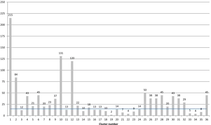
Fig. 6.

GNIP station data points per climatic cluster. The blue line indicates the minimum number of data

points (15) to successfully derive a M4 best-fit regression model for a given cluster.

35

Fig. 6. GNIP station data points per climatic cluster. The blue line indicates the minimum number of data points (15) to successfully derive

a M4 best-fit regression model for a given cluster.

values within a pair of data points (xandy, cf. Eq. 8):

2γ (x, y)= var (Z (x)−Z (y)) . (8)

The resulting semivariance of any particular point pair plot-ted against the distance between was used to create an empir-ical variogram, to which an experimental variogram model was fitted. The fitted function was defined by function type, nugget, sill, and range, and was used to predict values at any unknown location within a certain error range. Given the large heterogeneity of the GNIP data set (e.g., differ-ent scales for γ using different regression models, differ-ent months, stable isotopes), the recommended variogram autofitting function was augmented by a role-based defini-tion of the modeled variogram that “visually best fit” the point clouds. Briefly, our variograms were computed with a reasonable (for hydrologic purposes) cut-off lag distance of 150◦(e.g., data points located farther away than 150 spa-tial degrees from each other exerted no influence on the var-iogram). A robust variogram estimation was used (Cressie, 1993), whereby the width of the variogram bins was set to one-hundredth of the cut-off distance. An exponential func-tion was used to fit the point cloud. The nugget was set to the minimum ofγ, and sill was defined as the minimumγ

plus 2.25 times the standard deviation ofγ. The range was detected automatically when the curve function was fitted to the variogram data. This parameter setting was chosen to en-sure that any of the models tested (12 monthly for oxygen and hydrogen, plus one annual each, for both M1 and M4, in total 52) were subjected to the principles of identical treat-ment (PIT). When using the automatic parameter detection functions of the “gstat” library (Pebesma, 2004), some exper-imental variograms were found to be singular, with the model function not matching the curve given by the empirical

var-iogram. Hence, we used a parsimonious PIT approach that would not result in singular variograms. We are well aware that this conservative PIT approach might not result in a per-fect nugget/sill/range combination for each of the 52 models tested; however, comparability was maintained in all steps of the prediction/comparison workflow, which we deemed to be of greater importance for the RCWIP model comparison approach.

Kriging errors were calculated as the square root of the variance of the Kriging estimator as output by the “gstat” library. Kriging model evaluations were conducted by graph-ical and numergraph-ical comparisons of the variograms for the two core models (model M1 vs. M4). This is a rather simple approach to quantify the comparative outcomes of different geospatial models in order to determine which gives a better result; regression uncertainty may be incorporated as addi-tional uncertainty estimation into the future versions of the RCWIP model.

2.6 Confidence intervals

In order obtain a measure of the accuracy of the RCWIP re-gression and interpolation model prediction outcome, 95 % confidence intervals (CIs) were determined using the leave-one-out (n – 1) “jackknife” resampling procedure (Wu, 1986; Shao and Tu, 1995). The jackknifing method determined the robustness of model results by running ni iterations, each

time leaving one station data value out (i). In order to re-duce computational load, these calculations were restricted to a 2◦×2◦grid, which was sufficient for the determination of areas potentially deficient in predictive qualities.

Mathematically, the jackknife method was expressed

S. Terzer et al.: Global isoscapes forδ18O andδ2H in precipitation 4721

function ofδ18O (orδ2H), and in whichf (δ)encompasses both multiple regression and Kriging. A pseudo-value leav-ing out the stationiwas denoted as_θˆ

(i)=f (δ(−i)). We

cal-culated the mean_θˆ

J,x and standard error σ_θˆ

J,x of the

jack-knife for each grid cellxas the mean and standard deviation of the pseudo-values (Shao and Tu, 1995):

ˆ

θJ,x= n

P

i=1

ˆ

θ(i)

n , (9)

σ_θˆ_J,x= "

n−1

n

n

X

i=1

ˆ

θ(−i)− ˆθJ,x

2 #1/2

. (10)

The higher the standard error of the jackknife, the more vul-nerable a certain grid cell was to leaving that station data out. This standard error used for the computation of 95 % CIs was defined asc=(±)1.96σ_θˆ

J,x.

2.7 Data handling and numerical analysis

All isotopic, climatic, and geospatial data were collated in Microsoft Access databases. The model decision tree and geostatistical treatments were conducted using the R Statistical and Computing Environment (R Development Core Team, 2013) with the following package extensions: “RODBC”, “e1071”, “gstat” (Pebesma, 2004), and “rgdal”. Statistical evaluations were done using XLSTAT 2013 (www. xlstat.com). Plots were made using Grapher 10 (www. goldensoftware.com). All geospatial mapping was conducted using ArcGIS 2010 (www.ESRI.com, Redlands CA).

3 Results and discussion

3.1 Climatic clustering of GNIP stations

RCWIP’s data parameterization (i.e., minimum influence threshold, minimum ratio of remaining degrees of freedom over independent variables) required that any given climatic cluster domain needed mean values for a minimum of 15 GNIP stations for the computation of a cluster-specific re-gression model in model M4. Figure 6 shows the result of a histogram of the available data points per climatic cluster; the horizontal threshold line (n=15) could be compared to the minimum number of data points required for the computation of the regionalized model M4. This plot revealed that of the 36 climatic regions defined by fuzzy clustering, 15 zones did not meet the required data threshold for applying model M4. For these cases, model M2 was substituted by default. This graph further illustrated the relative paucity of isotopic data for specific spatial and climatic regions. For example, areas that were particularly data deficient in precipitation isotope data (up to 2009) to allow application of model M4 were climatic clusters 19 (western coast of Canada), 22 (western

Discussion

P

ap

er

|

Discussion

P

ap

er

|

Dis

cussion

P

ap

er

|

Discussion

P

ap

er

|

≤-5 -4 -3 -2 -1 0 1 2 3 4 >4

P oi n t co u n t Residuals (e) M4 (exc.kurt=3.79) M1 (exc.kurt=3.19) 0 20 40 60 80 100 120 140 160

-5.0 -4.5 -4.0 -3.5 -3.0 -2.5 -2.0 -1.5 -1.0 -0.5 0.0 0.5 1.0 1.5 2.0 2.5 3.0 3.5 4.0 4.5 5.0

P oi n t co u n t

Residuals' difference (Δe)

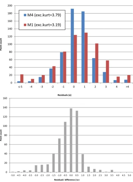
Fig. 7. (a)

Frequency histogram comparing the

δ

18

O

ANN

residuals of Model M1 and M4, as well as

excess kurtosis values.

(b)

Frequency histogram of the

δ

18

O

ANN

residuals’ difference between M4 and

M1 (

∆

e

=

e

M1

−

e

M4

;

n

= 623

). Values below zero indicate a lower residual in Model M4 versus Model

M1. The labels on the x-axis refer to the upper bin limit (i.e. 0.0 indicates

−

0.5

<

∆

e <

0.0)

36

Discussion

P

ap

er

|

Discussion

P

ap

er

|

Dis

cussion

P

ap

er

|

Discussion

P

ap

er

|

≤-5 -4 -3 -2 -1 0 1 2 3 4 >4

P oi n t co u n t Residuals (e) M4 (exc.kurt=3.79) M1 (exc.kurt=3.19) 0 20 40 60 80 100 120 140 160

-5.0 -4.5 -4.0 -3.5 -3.0 -2.5 -2.0 -1.5 -1.0 -0.5 0.0 0.5 1.0 1.5 2.0 2.5 3.0 3.5 4.0 4.5 5.0

P oi n t co u n t

Residuals' difference (Δe)

Fig. 7. (a)

Frequency histogram comparing the

δ

O

residuals of Model M1 and M4, as well as

excess kurtosis values.

(b)

Frequency histogram of the

δ

O

residuals’ difference between M4 and

M1 (

∆

e

=

e

−

e

;

n

= 623

). Values below zero indicate a lower residual in Model M4 versus Model

M1. The labels on the x-axis refer to the upper bin limit (i.e. 0.0 indicates

−

0.5

<

∆

e <

0.0)

36

Fig. 7. (a) Frequency histogram comparing theδ18OANNresiduals

of model M1 and M4, as well as excess kurtosis values. (b)

Fre-quency histogram of theδ18OANN residuals’ difference between

M4 and M1 (1e=eM1−eM4;n=623). Values below zero indicate

a lower residual in model M4 versus model M1. The labels on thex

axis refer to the upper bin limit (i.e., 0.0 indicates−0.5 <1e< 0.0).

USA), 33 (Pacific islands), and 34 (Australia). These and the 11 other identified areas could benefit from targeted new GNIP sampling efforts (Fig. 3). A map indicating the cover-age of M4 for annualδ18O is available from the Supplement (S5).

3.2 Evaluation of regression models

3.2.1 Residuals analysis

Comparing the residual statistics of model M4 versus M1 in Fig. 7a, several indicators of improved performance of model M4 were identified. The standard deviation of model M4 was lower than M1 (1.58 vs. 2.31), as was the interquartile range (1.57 vs. 2.51). The excess kurtosis of M4 exceeded that of M1 (3.79 vs. 3.19). The difference between model M1 and M4 residuals (1e=eM1−eM4;n=623) revealed that

4722 S. Terzer et al.: Global isoscapes forδ18O andδ2H in precipitation

Discussion

P

ap

er

|

Discussion

P

ap

er

|

Dis

cussion

P

ap

er

|

Discussion

P

ap

er

|

Cluster 01 – Berlin (Germany) Cluster 06 – Chiang Rai (Thailand)

Cluster 10 – Rabat/Kenitra (Morocco) Cluster 25 – Kingston (Jamaica)

Cluster 26 – Porto Nacional (Brazil) Cluster 32 – Honiara (Solomon Is.) 00 10 20 30 40 50 60 70 80 0 0.5 1 1.5 2 2.5 3 3.5 4

1 2 3 4 5 6 7 8 9 10 11 12

00 50 100 150 200 250 300 350 400 0 0.5 1 1.5 2 2.5 3 3.5 4

1 2 3 4 5 6 7 8 9 10 11 12

00 20 40 60 80 100 120 140 0 0.5 1 1.5 2 2.5 3 3.5

1 2 3 4 5 6 7 8 9 10 11 12

00 20 40 60 80 100 120 140 160 180 200 0 0.5 1 1.5 2 2.5 3 3.5 4 4.5 5

1 2 3 4 5 6 7 8 9 10 11 12

00 35 70 105 140 175 210 245 280 0 0.5 1 1.5 2 2.5 3 3.5 4

1 2 3 4 5 6 7 8 9 10 11 12

00 50 100 150 200 250 300 350 400 0 0.5 1 1.5 2 2.5 3 3.5 4

1 2 3 4 5 6 7 8 9 10 11 12

38

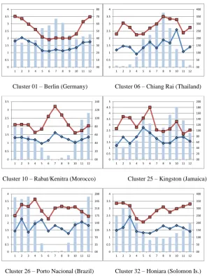
Fig. 8. Regression model (δ18O) performance comparison based on RMSE (‰, left axis) of models M1 (red) versus M4 (blue) for amount-weighted monthly predictions for six climatic cluster centroids. Lower RMSE means better performance. Mean monthly precipitation amount

(mm month−1, right axis) is shown by blue bars to indicate the timing of rainy and dry seasons. An ideal model would produce seasonally

consistently low RMSE. That there were flatter monthly patterns and a lower RMSE of M4 compared to M1 shows improved seasonal predictive outcomes when using regionalized best-fit regressor combinations.

M4 had lower residuals on average combined with a lower residual spread compared to M1.

3.2.2 Improved monthly predictions

The improved performance of model M4 in establishing re-gionalized precipitation isotope prediction models was par-ticularly evident when the time domain of the GNIP data was reduced to monthly means. The coefficient of determi-nation (R2)of the regression model for any particular month was limited by the fact there were fewer underlying data. For example, model M1 generally produced fairly highR2 val-ues overall, but it exhibited poorer performance in some ge-ographical areas like the tropics, and particularly when con-sidering monthly predictions. The root-mean-squared errors

(RMSE) of model M1 and M4 were examined for each cal-endar month and for each climatic cluster. The evaluations of all clusters revealed that the RMSE of model M4 was lower than M1 in all cases for bothδ18O andδ2H, in all 36 clus-ters for all 12 months, and in all clusclus-ters for the mean annual model. Comparisons for several selected climatic clusters are illustrated in Fig. 8. However, given the fragmented GNIP data coverage, it should be noted that suitable model M4 re-gression models could only be obtained for 56 and 58 % of theδ18O andδ2H combinations due to underlying data avail-ability constraints.

To illustrate the prediction precision outcomes, Fig. 8 shows the RMSE for model M1 versus M4 for mean monthly

S. Terzer et al.: Global isoscapes forδ18O andδ2H in precipitation 4723

Discussion

P

ap

er

|

Discussion

P

ap

er

|

Dis

cussion

P

ap

er

|

Discussion

P

ap

er

|

0 1 2 3 4 5 6 7 8

0 10 20 30 40 50 60 70 80 90 100 110 120 130 140 150

gam

m

a

(γ

)

Distance (degrees)

M1 (empirical) M1 (modeled) M4 (empirical) M4 (modeled)

Fig. 9.

Empirical (symbols) and the modeled (lines) variograms for

δ

O

of models M1 and M4.

Increased predictive precision (e.g. lower gamma values) over larger distances (x-axis) means better

performance.

40

Fig. 9. Empirical (symbols) and the modeled (lines) variograms forδ18OANNof models M1 and M4. Increased predictive precision (e.g.,

lower gamma values) over larger distances (xaxis) means better performance.

Discussion

P

ap

er

|

Discussion

P

ap

er

|

Dis

cussion

P

ap

er

|

Discussion

P

ap

er

|

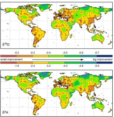
Fig. 10.A global map of the difference in prediction uncertainty between Models M1 and M4 (∆σ=

σM4−σM1)forδ18OANN(upper map, scale) andδ2HANN(lower map, scale), expressed in ‰. Stations

are indicated with “+” signs.

41

Fig. 10. A global map of the difference in prediction uncertainty

between models M1 and M4 (1σ =σM4−σM1)forδ18OANN

(up-per map, scale) andδ2H_ANN(lower map, scale), expressed in ‰.

Stations are indicated with “+” signs.

clusters 1, 6, 10, 25, 26, 32). The monthly RMSE patterns are underlain graphically by the monthly precipitation amounts. An ideal predictive isotope model would be seasonally flat and have a low RMSE. In all cases, model M4 obtained lower monthly RMSE values than model M1. In some cases, for example cluster 1 (Berlin), model M1 performed much more poorly in winter or, in the case of cluster 10 (Morocco), had the higher RMSE during the summer dry season. In short, the consistently overall lower RMSE of model M4 over M1 indi-cated that substantially improved seasonal and monthly pre-dictive outcomes were obtained using the RCWIP approach.

3.2.3 Interpolation

Following the analysis of the multivariate regression results, an evaluation of the performance of the interpolation meth-ods was undertaken. To achieve this, we examined the empir-ical and experimental semivariograms, along with the accom-panying interpolation uncertainty. For brevity, only models M4 versus M1 for amount-weighted annualδ18O (δ18OANN)

were illustrated. In Fig. 9, plots of the empirical and the-oretical variograms of δ18OANN for all GNIP stations are

4724 S. Terzer et al.: Global isoscapes forδ18O andδ2H in precipitation

Discussion

P

ap

er

|

Discussion

P

ap

er

|

Dis

cussion

P

ap

er

|

Discussion

P

ap

er

|

Fig. 11.

The 95 % CIs of Model M4 for mean

δ

H

in precipitation. The legend scale is

±

δ

H

expressed in ‰. The highest CIs (poorest performance) was clearly observed in the Himalayan region in

Asia. See text for discussion.

42

Fig. 11. The 95 % CIs of model M4 for meanδ2H_ANNin precipitation. The legend scale is±δ2H expressed in ‰. The highest CIs (poorest performance) are clearly observed in the Himalayan region in Asia. See text for discussion.

Discussion

P

ap

er

|

Discussion

P

ap

er

|

Dis

cussion

P

ap

er

|

Discussion

P

ap

er

|

Fig. 12.

Predicted global amount-weighted

δ

_O

ANN

of precipitation obtained using RCWIP. The legend

is

δ

O in ‰ relative to the VSMOW-SLAP scales.

43

Fig. 12. Predicted global amount-weightedδ18OANN of precipitation obtained using RCWIP. The legend isδ18O in ‰ relative to the

VSMOW-SLAP scales.

and clearly indicated superior performance over model M1 (±1.38 and±11.5 ‰, respectively). Outcomes for monthly prediction models and a table of the Kriging parameters are listed in Table S4.

Figure 10 shows a global map of the spatial distribution of the isotope prediction as the difference between predicted model outcomes of model M4 versus M1 (1σ=σM4−σM1)

for theδ18OANN andδ2HANN grids. The predicted isotope

differences varied spatially from little to no difference be-tween model M4 and M1 (e.g., < 0.2 ‰ forδ18O) to rather large differences (> 0.7 ‰ for δ18O). Model M4 outper-formed M1 particularly in data-scarce areas (e.g., in Aus-tralia, northern and central Asia, and Greenland), but also in parts of North America and Africa. On the other hand, any advantages to using RCWIP in isotope data-rich areas like Europe appeared to be limited (usually less than 0.3 ‰ difference, but see RMSE above).

3.3 Confidence intervals

The 95 % confidence intervals (CI) forδ18OANNandδ2HANN

models were derived as 1.96 times the standard error of the

S. Terzer et al.: Global isoscapes forδ18O andδ2H in precipitation 4725

P

ap

er

|

Discussion

P

ap

er

|

Dis

cussion

P

ap

er

|

Discussion

P

ap

er

|

Fig. 13.Comparison of difference (∆δ=δM4−δM1) in predicted amount weightedδ18OANN(upper

panel, scale) andδ2_H

ANN(lower panel, scale) comparing Model M1 and M4. The isotopic scale bar and

color scheme indicate the extent, positive or negative, and locations where M4 produced more positive or negative predicted values than M1.

44

Fig. 13. Comparison of difference (1δ=δM4−δM1)in predicted

amount-weighted δ18OANN (upper panel, scale) and δ2HANN

(lower panel, scale) comparing model M1 and M4. The isotopic scale bar and color scheme indicate the extent – positive or nega-tive – and locations where M4 produced more posinega-tive or neganega-tive predicted values than M1.

workflow, whereby data-deficient areas were covered by the globally parameterized regression model M2, whose size far exceeds any of the localized climatic subsets, and thereby precludes changes in the prediction result for any given jack-knifing pseudovalue. The data scarcity limitation applies, for example, to climatic clusters 16 and 18–24 (North America), 11 and 14 (western and central Africa), 34 and 35 (Australia, New Zealand), and 3 (Russia). It was anticipated that 95 % CIs may be further improved through the targeted collec-tions of new precipitation isotope data in these regions into the future.

3.4 Global precipitation isoscape maps

The final outcome of the RCWIP approach was to construct globally gridded precipitation prediction maps (isoscape maps) ofδ18O andδ2H for the Earth’s land areas (exclud-ing Antarctica), restricted to a 10 arcmin resolution. These isoscape map products included precipitation δ18OANN

andδ2HANN, amount-weighted growing-seasonδ18OGSand

δ2HGS, and amount-weighted monthly grids. A complete

suite of isoscape map products has been made available for public use as geo-referenced TIFF (GeoTIFF) files, avail-able from the website of the IAEA Water Resources Program (www.iaea.org/water/). These GeoTIFF files can be used in a variety of disciplinary fields of hydrologic and ecological research.

To provide a few comparative outcome examples, the pre-dicted global isoscape map forδ18OANNwas determined

us-ing the RCWIP approach, and is depicted in Fig. 12. In order compare the RCWIP approach to model M1, a map show-ing the isotopic difference (1δ)for δ18OANN andδ2HANN

was constructed, and is illustrated in Fig. 13. Examination of Fig. 13 reveals several substantial differences between RCWIP and model M1, in some cases for only one of the iso-topes. One of the most obvious differences between RCWIP and model M1 for both isotopes was found in the Arctic re-gions – particularly Greenland – and for parts of northern Asia (e.g., Siberia). In these areas, RCWIP consistently pro-duced more negativeδ2OANN andδ2HANN predictions for

precipitation. To a lesser extent, this also held true for the western Andes and for parts of northern Africa, particularly the Ethiopian Highlands (Fig. 13). Conversely, RCWIP pro-duced more positiveδ18OANNandδ2HANNpredictions than

model M1 in Australia and the Himalayas, as well as over parts of eastern Asia, to a lesser extent over southwestern North America, and in parts of the South American lowlands and the Arabian Peninsula (Fig. 13).

Decoupled isotopic differences (e.g., more enriched or de-pleted in18O than2H than was expected from the GMWL relationship) in the results of RCWIP compared to model M1 were observed over the Tibetan Plateau, over the Andes, and in the northern Sahara (Fig. 13). These “decoupled” isotopic differences generally occurred for climatic cluster domains for which there were sufficient isotope data to build climate-cluster-specific M4 regression models for only the one but not for the other isotope (e.g., Fig. 3), especially climatic clusters 7, 8, and 29. This observation was corroborated by correspondingly higher CIs in these same areas (Fig. 11). We therefore caution isoscape map users, particularly those working in the geographical areas listed here, to carefully verify these model results with data in these areas.

Finally, there is tremendous interest in precipitation hy-drogen and oxygen isoscape maps for use in forensics and plant and food authenticity, as well as in wildlife and eco-logical studies. Previous research showed that the δ2H of plant and wildlife tissue generally showed the strongest cor-relation with amount-weighted growing-season precipitation

4726 S. Terzer et al.: Global isoscapes forδ18O andδ2H in precipitation

Discussion

P

ap

er

|

Discussion

P

ap

er

|

Dis

cussion

P

ap

er

|

Discussion

P

ap

er

|

Fig. 14.

Predicted amount-weighted mean growing season

δ

_H

GS

in precipitation obtained using

RCWIP. Growing season was defined as the mean of all months where the average air temperature was

>

0

C. Legend is

δ

_{H in ‰, relative to VSMOW-SLAP scales.}

45

Fig. 14. Predicted amount-weighted mean growing-seasonδ2HGSin precipitation obtained using RCWIP. Growing season was defined as

the mean of all months where the average air temperature was > 0◦C. Legend isδ2H in ‰, relative to VSMOW-SLAP scales.

4 Conclusions and outlook

A new regionalized cluster-based water isotope prediction (RCWIP) approach based on over 50 yr of GNIP data was demonstrated for the purposes of predicting spatio-temporal patterns of the stable isotope composition (δ2H,δ18O) of pre-cipitation around the world. Through the use of statistically defined climatic spatial domains, a series of flexible climatic and spatial explanatory regressor variables were used for test-ing all available models (global–regional to fixed–flexible regressors) in order to obtain the best predictive model for each climatic cluster. The best individual cluster-optimized prediction models were seamlessly amalgamated into single global map products by using fuzzy clustering. Compara-tive tests revealed that the RCWIP approach outperformed the previously well-established model M1 > 67 % of the time, and furthermore clearly improved both our predictive accu-racy and precision. The main outcome of the RCWIP ap-proach was to produce improved generalized and discipline-specific relevant and useful precipitation isoscape map prod-ucts to be available for download and public use from the IAEA website.

Some precautionary notes on the use of δ2H and δ18O isoscape predictive maps must be emphasized. As noted, pre-cipitation isoscape mapping products were based upon dis-continuous long-term data sets within the GNIP database, and therefore these mapping efforts had an inherent assump-tion of temporal constancy in their predictive outcomes, which may not be true for some regions of the world. For many applications, small overall time changes in precipita-tion isotopes were not likely to be strongly manifested in some receiving environments of interest. Groundwater, for example, tended to reflect precipitation events averaged over years to decades, and so would be slowly responsive to cli-matically driven or stochastic weather events and isotopic changes. For other disciplines where there was a strong in-terest in precipitation isoscapes (e.g., plant or animal ecol-ogy, food authenticity), there may be highly relevant

interan-nual, stochastic, or seasonal differences in the precipitation regimes (wet/dry years, ENSO) that could affect the amount of “relevant” precipitation water entering the soil, food webs, and biological and plant tissues (and possibly also affected the isotopic composition). For those disciplines where the timescales of “which water matters” was critical, the use of isoscape map products may be useful as a first-order starting point for predictive modeling, but should be used with great caution and need to be tested and validated (e.g., annual cal-ibrations with GNIP data).

Regarding spatial and temporal data coverage, RCWIP provided a strong and a flexible platform for predicting pre-cipitation isoscapes, although modeling efforts were only as good as the supporting foundational data pillars. Spatial gaps in precipitation isotope collected data at global scales, spa-tially and temporally, over many decades were inevitable. Here, the climatic fuzzy clustering of GNIP stations allowed us to identify particularly relevant and data-deficient areas of the world. RCWIP thereby provided a basis upon which to better inform future volunteer efforts in contributing to the GNIP database. In particular, new multiyear efforts of strate-gically located GNIP collections would be useful in certain areas of Africa, central Asia, and in South America.

Supplementary material related to this article is

available online at http://www.hydrol-earth-syst-sci.net/ 17/4713/2013/hess-17-4713-2013-supplement.zip.

Acknowledgements. The authors are indebted to the numerous and

invaluable voluntary contributors of precipitation stable isotopic data to the GNIP database over the past 60 yr from many countries. Funding for this research was provided by the International Atomic Energy Agency.

Edited by: C. Stumpp

References

Aggarwal, P., Araguas, L., Groening, M., Kulkarni, K. M., New-man, B. D., and Vitvar, T.: Global hydrological isotope data net-works, in: Isoscapes: Understanding movement, pattern, and pro-cesses on Earth through isotope mapping, edited by: West, J. B., Bowen, G. J., Dawson, T. E., and Tu, K. P., Springer, 330050, 2010.

Aggarwal, P. K., Alduchov, O. A., Froehlich, K. O., Araguas-Araguas, L. J., Sturchio, N. C., and Kurita, N.: Stable isotopes in global precipitation: A unified interpretation based on at-mospheric moisture residence time, Geophys. Res. Lett., 39, L11705, doi:10.1029/2012GL051937, 2012.

Bezdek, J.: Pattern Recognition With Fuzzy Objective Function Al-gorithms, Plenum, New York, 1981.

Birks, S., Gibson, J., Gourcy, L., Aggarwal, P., and Edwards, T.: Maps and animations offer new opportunities for studying the global water cycle, EOS T. Am. Geophys. Un., 83, p. 406, doi:10.1029/2002EO000298, 2002.

Bowen, G. J.: Statistical and geostatistical mapping of precipita-tion water isotope ratios, in: Isoscapes: Understanding move-ment, pattern, and process on Earth through isotope mapping, edited by: West, J. B., Bowen, G. J., Dawson, T. E., and Tu, K. P., Springer, London, 139–178, 2010.

Bowen, G. J. and Revenaugh, J.: Interpolating the isotopic compo-sition of modern meteoric precipitation, Water Resour. Res., 39, 1299, doi:10.1029/2003WR002086, 2003.

Bowen, G. J. and Wilkinson, B.: Spatial distribution ofδ18O in

me-teoric precipitation, Geology, 30, 315–318, 2002.

Bowen, G. J., Wassenaar, L. I., and Hobson, K. A.: Global applica-tion of stable hydrogen and oxygen isotopes to wildlife forensics, Oecologia, 143, 337–348, 2005a.

Bowen, G. J., Winter, D. A., Spero, H. J., Zierenberg, R. A., Reeder, M. D., Cerling, T. E., and Ehleringer, J. R.: Stable hydrogen and oxygen isotope ratios of bottled waters of the world, Rapid Com-mun. Mass Sp., 19, 3442–3450, 2005b.

Cannon, R. L., Dave, J. V., and Bezdek, J. C.: Efficient Implemen-tation of the Fuzzy c-Means Clustering Algorithms, IEEE T. Pat-tern Anal., 8, 248–255, 1986.

Clark, I. D. and Fritz, P.: Environmental Isotopes in Hydrogeology, Lewis Publishers, New York, 328 pp., 1997.

Cormie, A. B., Schwarcz, H. P., and Gray, J.: Relation between hy-drogen isotopic ratios of bone collagen and rain, Geochim. Cos-mochim. Ac., 58, 377–391, 1994.

Craig, H.: Isotopic Variations in Meteoric Waters, Science, 133, 1702–1703, doi:10.1126/science.133.3465.1702, 1961. Cressie, N. A.: Statistics for Spatial Data, Wiley & Sons, New York,

1993.

Dansgaard, W.: The18O Abundance in Fresh Water, Geochim.

Cos-mochim. Ac., 6, 241–260, 1954.

Dansgaard, W.: Stable isotopes in precipitation, Tellus, 5, 436–468, 1964.

Delavau, C., Stadnyk, T., and Birks, J.: Model Based Spatial Dis-tribution of Oxygen-18 Isotopes in Precipitation Across Canada, Can. Water Resour. J., 36, 313–330, 2011.

Delhomme, J. P.: Kriging in the Hydrosciences, Adv. Water Resour. Res., 1, 251–266, 1978.

Dutton, A., Wilkinson, B. H., Welker, J. M., Bowen, G. J., and Lohmann, K. C.: Spatial distribution and seasonal variation in

18_O/16_{O of modern precipitation and river water across the}

con-terminous USA, Hydrol. Process., 19, 4121–4146, 2005. Ehleringer, J. R., Bowen, G. J., Chesson, L. A., West, A. G.,

Podle-sak, D. W., and Cerling, T. E.: Hydrogen and oxygen isotope ratios in human hair are related to geography, P. Natl. Acad. Sci. USA, 105, 2788–2793, 2008.

Epstein, S. and Mayeda, T.: Variation of18O content of waters from

natural sources, Geochim. Cosmochim. Ac., 4, 213–224, 1953.

Fraser, I. and Meier-Augenstein, W.: Stable2H isotope analysis

of human hair and nails can aid forensic human identification, Rapid Commun. Mass Sp., 21, 3279–3285, 2007.

Friedman, I.: Deuterium content of natural waters and other sub-stances, Geochim. Cosmochim. Ac., 4, 89–103, 1953.

Froehlich, K. F. O., Gonfiantini, R., and Rozanski, K.: Isotopes in Lake Studies: A Historical Perspective, in: Isotopes in the Water Cycle: Past, present and future of a developing science, edited by: Aggarwal, P. K., Gat, J., and Froehlich, K. F. O., Springer Netherlands, 139–150, 2005.

International Atomic Energy Agency/World Meteorological Orga-nization (IAEA/WMO): Global Network of Isotopes in Precipita-tion, The GNIP Database, available at: http://www.iaea.org/water (last access: 23 March), 2013.

Heaton, K., Kelly, S. D., Hoogewerff, J., and Woolfe, M.: Verifying the geographical origin of beef: The application of multi-element isotope and trace element analysis, Food Chem., 107, 506–515, 2008.

Hobson, K. A. and Wassenaar, L. I.: Linking brooding and winter-ing grounds of neotropical migrant songbirds uswinter-ing stable hy-drogen isotopic analysis of feathers, Oecologia, 109, 142–148, 1997.

Kendall, C. and McDonnell, J. J.: Isotope tracers in catchment hy-drology, Elsevier Science Limited, 1998.

Kottek, M., Grieser, J., Beck, C., Rudolf, B., and Rubel, F.: World map of the Koppen-Geiger climate classification updated, Mete-orol Z., 15, 259–263, 2006.

Kralik, M., Papesch, W., and Stichler, W.: Austrian Network of Iso-topes in Precipitation (ANIP): Quality Assurance and Climato-logical Phenomenon in one of the Oldest and Densest Networks in the World, in: Isotope Hydrology and Integrated Water Re-sources Management, IAEA, Vienna, 146–149, 2003.

4728 S. Terzer et al.: Global isoscapes forδ18O andδ2H in precipitation

Liebminger, A., Haberhauer, G., Papesch, W., and Heiss, G.: Corre-lation of the isotopic composition in precipitation with local con-ditions in alpine regions, J. Geophys. Res.-Atmos., 111, D05104, doi:10.1029/2005JD006258, 2006.

Liu, Z., Tian, L., Chai, X., and Yao, T. D.: A model-based

deter-mination of spatial variation of precipitationδ18O over China,

Chem. Geol., 249, 203–212, 2008.

Lykoudis, S. P. and Argiriou, A. A.: Gridded data set of the sta-ble isotopic composition of precipitation over the eastern and central Mediterranean, J. Geophys. Res.-Atmos., 112, D18107, doi:10.1029/2007JD008472, 2007.

Matheron, G.: Principles of Geostatistics, Econ. Geol., 58, 1246– 1266, 1963.

McBratney, A. B. and Moore, A. W.: Application of Fuzzy-Sets to Climatic Classification, Agr. Forest Meteorol., 35, 165–185, 1985.

New, M., Lister, D., Hulme, M., and Makin, I.: A high-resolution data set of surface climate over global land areas, Clim. Res., 21, 1–25, 2002.

Pebesma, E. J.: Multivariable geostatistics in S: the gstat package, Comput. Geosci., 30, 683–691, 2004.

Peterson, T. C., Vose, R., Schmoyer, R., and Razuvaev, V.: Global historical climatology network (GHCN) quality control of monthly temperature data, Int. J. Climatol., 18, 1169–1179, 1998.

Popa-Lisseanu, A. G., Sorgel, K., Luckner, A., Wassenaar, L. I., Ibanez, C., Kramer-Schadt, S., Ciechanowski, M., Gorfol, T., Niermann, I., Beuneux, G., Myslajek, R. W., Juste, J., Fonder-flick, J., Kelm, D. H., and Voigt, C. C.: A Triple-Isotope Ap-proach to Predict the Breeding Origins of European Bats, PLoS One, 7, e30388, doi:10.1371/journal.pone.0030388, 2012. R Development Core Team: R: A language and environment for

statistical computing, R Foundation for Statistical Computing, Vienna, available at: http://www.R-project.org/, 2013.

Rozanski, K.: Deuterium and18O in European groundwaters – links

to atmospheric circulation in the past, Chem. Geol., 52, 349–363, 1985.

Rozanski, K., Araguas-Araguas, L., and Gonfiantini, R.: Isotopic patterns in modem global precipitation, in: Climate Change in Continental Isotopic Records – Geophysical Monograph 78, edited by: Swart, P. K., Lohman, K. C., McKenzie, J., and Savin, S., American Geophysical Union, Washington, DC, 1–36, 1993. Shao, J. and Tu, D.: The Jackknife and Bootstrap, Springer, New

York, 1995.

Sheppard, S. M., Nielsen, R. L., and Taylor, H. P.: Oxy-gen and HydroOxy-gen Isotope Ratios of Clay Minerals from

Porphyry Copper Deposits, Econ. Geol., 64, 755–777,

doi:10.2113/gsecongeo.64.7.755, 1969.

Soto, D. X., Wassenaar, L. I., and Hobson, K. A.: Stable hydro-gen and oxyhydro-gen isotopes in aquatic food webs are tracers of diet and provenance, Funct. Ecol., 27, 535–543, doi:10.1111/1365-2435.12054, 2013.

van der Veer, G., Voerkelius, S., Lorentz, G., Heiss, G., and Hoogewerff, J. A.: Spatial interpolation of the deuterium and oxygen-18 composition of global precipitation using temperature as ancillary variable, J. Geochem. Explor., 101, 175–184, 2009. Wang, C.-H. and Peng, T.-R.: Hydrogen and Oxygen Isotopic

Com-positions of Taipei Precipitation 1990 to 1998, Western Pacific Earth Sciences, 1, 429–442, 2001.

Wassenaar, L. I., Van Wilgenburg, S. L., Larson, K., and Hobson, K.

A.: A groundwater isoscape (δD,δ18O) for Mexico, J. Geochem.

Explor., 102, 123–136, 2009.

Welker, J. M.: ENSO effects onδ18O,δ2H and d-excess values in

precipitation across the U.S. using a high-density, long-term net-work (USNIP), Rapid Commun. Mass Sp., 26, 1893–1898, 2012. World Meteorological Organization (WMO): Guide to Meteorolog-ical Instruments and Methods of Observation, 7th Edn., World Meteorological Organization, Geneva, 2008.

Wu, C. F. J.: Jackknife, Bootstrap and Other Resampling Methods in Regression-Analysis – Rejoinder, Ann. Stat., 14, 1343–1350, 1986.