Work Package 2 – Review of Environmental and Transportation Modelling
Methods and Development of Transport Emissions Model
Deliverable D2.1 – Technical report detailing the research conducted in WP2. Literature
review of transportation models. Deadline Month 12
Authors
Páraic Carroll - Trinity College Dublin
Shreya Dey - Trinity College Dublin
Brian Caulfield - Trinity College Dublin
Francesco Pilla - Trinity College Dublin
Bidisha Ghosh - Trinity College Dublin
Aoife Ahern – University College Dublin
Edgar Morgenroth – ESRI
May 2016
i
Table of Contents
Section 1: Examining the most appropriate Transportation Models
and Data
1
1.1 Introduction
1
1.2 Transportation Models for Ireland
2
1.2.1 NTA Model
2
1.2.2 TII Model
6
1.2.3 ESRI HERMES
9
1.2.4 ESRI ISus
12
1.2.5 UCD MOLAND
15
1.3 DTTaS Common Appraisal Framework for Transport Projects and
Programmes
18
1.4 International Best Practice
20
Section 2: Examining the most appropriate Environmental Models
and Data
25
2.1 Introduction
25
2.1.1 Classification of emission model
25
2.2 The Existing Emission Modelling Tools
26
2.2.1 ARTEMIS
26
2.2.2 COPERT
27
2.2.3 HBEFA
28
2.2.4 MOBILE
31
2.2.5 MOVES
31
2.2.6 NAEI
32
2.2.7 PHEM
32
2.2.8 TREMOD
32
2.2.9 VEPM
33
2.2.10 VFEM
33
2.2.11 VERSIT+
33
2.3 Transportation Emission Model for Ireland
34
2.3.1 Executive Review of COPERT 4
34
2.3.2 COPERT 4 in Ireland
35
2.4 COPERT 4: Elements and Properties
35
2.4.1 COPERT 4: Software development and Use
35
2.4.2 Properties of COPERT4
37
2.4.3 Major individual application
37
2.4.4 Input parameters
37
2.4.5 Expected Results
44
2.4.6 Additions in COPERT 5
45
ii
3.1 Discussion and Conclusion
46
3.2 The Transport Emissions Model
47
iii
List of Tables
Table 1: NTA Model
2
Table 2: TII Model
6
Table 3: ISus Model
12
Table 4: MOLAND Model
15
Table 5: DTTaS Transport Parameter Values
19
Table 6: Key Elements from the Models
23
Table 7: Emission models
26
Table 8: Various relevant emissions models
29
Table 9: Sources of COPERT 4 input data
43
Table 10: Technology class of different vehicles
43
Table 11: Importance and availability of statistics of different
iv
List of Figures
Figure 1: GDA Model Structure
4
Figure 2: TII Model Structure
7
Figure 3: Choice Structure of the Variable Demand Model
8
Figure 4: Key mechanisms within the HERMES model
10
Figure 5: Flowchart of ISus
13
Figure 6: MOLAND Model Structure
16
Figure 7: UK NTM Model Structure
20
Figure 8: Sweden SAMPERS Model Structure
22
Figure 9: The European Topic Centre on Air Pollution and Climate Change
Mitigation (ETC/ACM)
35
Figure 10: Distribution of different model usage for transportation-emission
calculation
36
Figure 11: Continent wise distribution of COPERT application
36
Figure 12: COPERT application in different areas
36
Figure 13: Screenshot of COPERT 4: Meteorological information
38
Figure 14: Screenshot of COPERT 4: Fleet configuration
38
Figure 15: Screenshot of COPERT 4: Activity Data
39
Figure 16: Screenshot of COPERT 4: Circulation Data
40
Figure 17: Screenshot of COPERT 4: Evaporation Data
40
Figure 18: Screenshot of COPERT 4: Output forms for Hot emission
41
Figure 19: Screenshot of COPERT 4: Output forms for cold start emission
42
Figure 20: Flowchart of Transport Emissions Model
42
Figure 21. Instrumental set up
46
Figure 22: Current Scenario
48
1
Section 1: Examining the most appropriate Transportation Models and Data
1.1 Introduction
This deliverable provides an extensive overview of a selection of relevant economic, environmental, land-use and transportation models currently available in the Republic of Ireland and internationally that have been designated as being appropriate for use in research in the Greening Transport Project. The models were deemed suitable by the project team due to the methods that they employ, the nature of the inputs that are included in the models and most importantly based upon the utility of the outputs generated. It is the key goal of the Greening Transport Project to develop a Transport Emissions Model capable of combining transportation modelling practices with the outputs generated from an emission model (Task 2.2) to accurately analyse the effect of behavioural and policy changes on greenhouse gas emissions from transport in Ireland. In this way, the outputs from the selected models will be fed into the newly developed model to effectively inform policymaking decisions on a regional and national level and to provide the basis for further research conducted as part of the project.
The transport-related models that have been reviewed are:
(1) The National Transport Authority (NTA) Greater Dublin Area (GDA) Model; (2) Transport Infrastructure Ireland (TII) National Transport Model (NTpM);
(3) The Economic and Social Research Institute’s (ESRI) HERMES (Harmonized Economic Research Models on Energy Systems);
(4) ISus (Irish Sustainable Development Model) models and finally;
2
1.2 Transportation Models for Ireland
1.2.1 The NTA Greater Dublin Area Model
The first iteration of the NTA model was developed in 1991 as part of the Dublin Transportation Initiative (DTI) study and in 1996 the Dublin Transportation Office (DTO) (subsumed into the NTA in December, 2009) took ownership of the model which has since undergone a number of updates with input from external consultants. One such consultant was Steer Davies Gleave who in 2008 were commissioned to aid in the update and re-calibration of the model, results of which have been detailed in a number of model calibration reports (DTO and Steer Davies Gleave, 2009). National Transport Authority (NTA) is the main government funded entity responsible for a range of transportation functions in Ireland including: transport planning and investment in the GDA, national public transport delivery and bus and taxi regulation, the NTA accordingly has the most comprehensive bank of transportation data in Ireland. As a result of this, the NTA’s foremost transportation model: the Greater Dublin Area Model which has been central to the Draft Transport Strategy 2011-2030 in addition to the proposed GDA Transport Strategy 2015-2035 and Dublin City Development Plan; has been identified as being the most suitable for the nature of the research conducted in Greening Transport Project. An overview of the inputs and outputs of the NTA GDA Model are presented in Table 1 below.
Table 1: NTA Model
Inputs Outputs
Place of Work and School Census of Anonymised Records (POWSCAR)
Trip Generation – estimation and prediction of the number of trips generated by and attracted to a zone (travel demand) by purpose (commuting, education, business, etc.)
GDA Travel to Education Survey Trip Distribution - Patterns of trips between sets of trip generators and trip attractions (trip ends)
GDA Household Survey Car Ownership Model – car ownership trends over time, determination of the probability of car availability for a particular trip (i.e. car available/ not available)
CSO Small Area Population Statistics
(SAPS) datasets Mode Choice – trips matrices split into different modes of travel (car, public transport and active modes i.e. walking and cycling)
Hour of Travel Choice (AM Peak only) – trips further split down to the hour of travel (7-8:00, 8-9:00, 9-10:00)
Macroeconomic forecasts and Regional Planning Guidelines (RPG) to determine travel demand into the future (i.e. target year 2030)
Trip assignment to their respective (road or public transport networks)
3 Macroeconomic forecasts and Regional Planning Guidelines (RPG) are the main determinants of travel demand in the 2030 target year, the ESRI (HERMES and ISus) and the UCD MOLAND models are crucial in this respect. It is comprised of 666 zones (657 internal fine zones covering the
modelled area and 9 external zones representing travel between the modelled area and the rest of Ireland) (NTA, 2012).
Model Structure: The current GDA Model was created following the 2008 Dublin Transport Authority (DTA) Act’s (Section 12) plan to develop a Draft Transport Strategy for the NTA Eastern Regional Model (ERM)/ Greater Dublin Area consisting of the counties of Dublin, Meath, Kildare and Wicklow. It covers the morning (AM Peak) period between 07:00 and 10:00 and the afternoon Off/ Inter-Peak period between 14:00 and 15:00. The ERM is one of five other regional models operated by the NTA (South East Regional Model, South West Regional Model, Mid-West Regional Model and the Western Regional Model). The model contains coded networks for all networks for all mechanised modes of travel – including car, HGV, heavy rail and Luas (NTA, 2012).
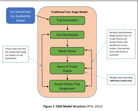
The AM Peak and Off Peak period differ slightly in their structure as the AM Peak includes an extra component: ‘Hours of Travel Choice’. This is only relevant to the AM Peak as it is used to “model the impacts of peak spreading where people decide to depart at an earlier (or later) time to avoid congestion or crowding during the morning peak” (NTA, 2012). The GDA AM Peak Model continuously iterates between the mode choice, time of travel choice and trip assignment stages of model until an equilibrium of travel costs across travel modes, time periods and travel routes is achieved. Travel costs derived from the trip assignment stage can also impact on trip distribution. The Off Peak Model follows the Traditional Four Stage Model (FSM) as it simply relates to a one hour period that isn’t usually affected by peak spreading. The model is displayed in Figure 1 below.
The GDA Model organises travel demand in the form of six journey purposes: Work (commuting), Education, Employer’s Business, Shopping, Other and Non-Home Based and for each of these journey purposes travel demand is segmented into a Car Available and Car Not Available groups, this represents the purpose of the Car Ownership/ Car Availability Model. This model feeds into the Trip Generation stage and it tracks and predict growth in car ownership over time and determines the probability of people in a particular zone owning a car.
4
Figure 1: GDA Model Structure (NTA, 2012)
Critical Analysis of the NTA GDA Model
Pros: A wide range of stakeholders, partners and other parties can make use of the model ensuring maximum possible dissemination of model outputs and increasing the productivity associated with it.
The model includes trips by all the main modes of travel – including trips by walking and cycling. These actives modes are of particular interest in the context of the project as they represent a viable, sustainable and smart alternatives to private car travel, especially in urban areas.
Travel behaviour is based on comprehensive and detailed travel surveys and travel datasets not generally available in strategic models elsewhere. By studying behavioural changes and restraints in this respect our research will be capable of examining the steps needed to induce emissions reductions as result of such behavioural shifts.
The model covers the GDA, and takes full account of travel within, into and out of the modelled area. The GDA is of substantial national importance in terms of sustaining the economic competitiveness of Ireland and attracting international investment which plays a vital part in driving economic prosperity in the country.
Trip Generation
Trip Distribution
Mode Choice
Hours of Travel Choice
Route Choice/ Trip Assignment Car Ownership/
Car Availability Model
Iteration loop between Mode Choice, Hour of Travel Choice and Route Choice until equilibrium across modes, time periods and route choice is achieved
Models peak spreading (AM-Peak model only) Travel costs from the
trip assignment stage can impact on trip distribution
5 To enhance its functionality, the GDA transport model includes an additional stage (‘hour of travel choice’) in the modelling process. As stated before, this additional stage is used to represent the phenomenon of peak spreading as a response to congestion and is not captured in many strategic models of this kind. By studying peak spreading it provides a further level of scope to the analysis of trip decision making which in this way, highlights areas of low accessibility to public transport services or fleet management issues such as poor fleet capacity during peak hours.
Peak Spreading highlights the advantages of taking active modes of transport to avoid this problem – for this reason active modes are not included in the Hour of Travel Choice stage of the model
Cons:
The model doesn’t include car sharing, carpooling, taxi/ on demand services (Uber/ Hailo) that are examples of sustainable and efficient use of resources which have an effect on reducing road congestion and encourage higher occupancy of cars. Taxis are only treated as cars and are not separated as an individual mode in itself. Thus, given the growth and popularity of on-demand services like Hailo/ Uber, it is necessary to include these services in updated versions of the model.
Though walking and cycling trips are included in the model, they are not assigned to equivalent walking and cycling networks. Hence, whereas the cost of travel by mechanised modes is based on travel demand and network characteristics, the cost of travel for non-mechanised modes is calculated as a simple combination of travel time and distance. The model is thus limited in its ability to test policies that seek to increase trips by walking and cycling. In particular, the model cannot automatically capture the time savings and other user benefits accruing to pedestrians and cyclists as a result of priority and other network improvements that confer advantages on these modes (NTA, 2012).
Walkability maps or audits and walk and cycling networks must be created and integrated into the model in order to fully take account of the assignment of active travel modes in the GDA which are growing thanks to schemes like the Dublin Bikes. This may help to highlight the cost benefit analysis of investing more financial resources into our walking and cycling infrastructure to further encourage these sustainable modes, particularly in suburban and rural areas where transport by means of the privately owned car is the safest and sometimes the only form of transport.
There is no reference to carbon trajectories which could be linked to travel demand patterns on road and public transport networks in order to bring about closer integration between transport and emissions estimates. Examples of this can be taken from Great Britain in the period of 1999-2001 (UK NTM) where emissions targets and carbon trajectories have been combined with transport modelling processes to generate greater coordination on this issue (WSP, 2011). A larger focus on urban environmental impacts and accessibility to public transport should be
built into our transport modelling practices. An example of which can be taken from Sweden in the Early 1980s (WSP, 2011). This is ultimately the aim of the Greening Transport Project
6
1.2.2 TII National Transport Model (NTpM)
Transport Infrastructure Ireland (TII) has the responsibility for securing a safe and efficient network of national roads in the Republic of Ireland. It commissioned the development of the National Traffic Model (NTM) completed in 2008, which was subsequently enhanced in 2010 and 2011 to include the
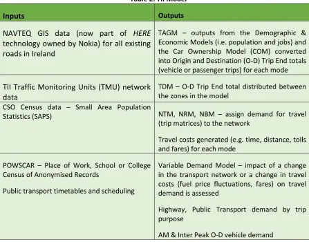
[image:11.595.68.516.209.559.2]National Rail Model, National Bus Model and a Variable Demand Model. An overview of the inputs and outputs of the TII NTpM Model are outlined in Table 2 below that include the sub-models stated.
Table 2: TII Model
Inputs
OutputsNAVTEQ GIS data (now part of
HERE
technology owned by Nokia) for all existing
roads in Ireland
TAGM – outputs from the Demographic & Economic Models (i.e. population and jobs) and the Car Ownership Model (COM) converted into Origin and Destination (O-D) Trip End totals (vehicle or passenger trips) for each mode
TII Traffic Monitoring Units (TMU) network
data
TDM – O-D Trip End total distributed between the zones in the model
CSO Census data – Small Area Population
Statistics (SAPS) NTM, NRM, NBM – assign demand for travel (trip matrices) to the network
Travel costs generated (e.g. time, distance, tolls and fares) for each mode
POWSCAR – Place of Work, School or College Census of Anonymised Records
Public transport timetables and scheduling
Variable Demand Model – impact of a change in the transport network or a change in travel costs (fuel price fluctuations, fares) on travel demand is assessed
Highway, Public Transport demand by trip purpose
AM & Inter Peak O-D vehicle demand
The full model that contains all of these modules is what constitutes the National Transport Model (NTpM), the structure of which is illustrated in Figure 2 below (NRA et al., 2014)
7
Figure 2: TII Model Structure (NRA et al., 2014)
The NTpM is linked to the NTA GDA Model by means of using many of the models that the GDA Model employs, such as the COM, Trip Attraction and Generation Model (TAGM) and the Trip Distribution Model however it uses these models on a national scale as opposed to a regional scale. The fundamental function of the NTpM is to “support and complement the existing and planned urban area transport models that are in use, or will be used by authorities in Dublin, Cork, Limerick, Waterford and Galway” (NRA et al., 2014). The NTpM models inter-city/inter-urban public transport and road networks which are not included in urban area transport models.
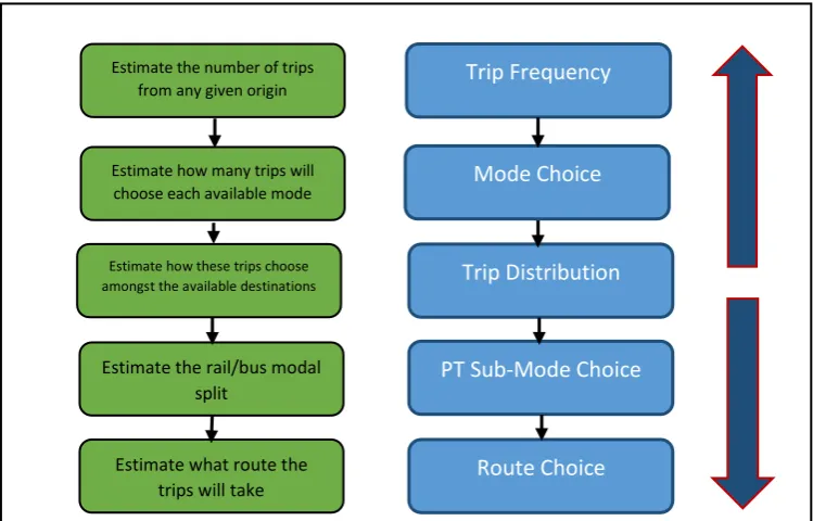
The Variable Demand Model (VDM) is the central tool of the model suite which interfaces with the highway and public transport elements of the NTpM developed using Python programming and VISUM modelling software (AECOM et al., 2012). It simulates a ‘Do Minimum’ scenario whereby the least possible action taken is compared with a ‘Do Something’ where the maximum amount of action is executed. Multiple regression analysis is the method used to produce forecast trip ends. The costs changes of both scenarios are the subject of the comparison which occurs when model calculations for variable demand are executed. Similarly to the NTA model, the NTpM performs the calculations based on the AM and Inter Peak periods for the Road, Rail and Bus Assignment Models, the same trip purposes (work, education, shopping, leisure etc.) and the car availability groups are also employed as a reference demand in the trip matrices.
In addition to the COM, TAGM, and TDM, the VDM is supplemented by a range of economic and modelling parameters, namely: fuel efficiency and consumption, vehicle occupancy, trip frequency and proportions of travel from home which are required for each trip purpose. This data is then fed into the traffic, road/ highway and public transport assignment models before being passed onto the VDM for the travel demand to be calculated and processed. The VDM process can be seen in Figure 3 below.
NTpM
Variable Demand Model (VDM)
NTM NRM NBM
Demographic &
8
Figure 3: Choice Structure of the Variable Demand Model (AECOM et al., 2012).
Critical Analysis of the TII Model
Pros: The NTpM provides a high level of functionality, allowing for the following responses to be assessed:
- Changes in traffic assignment due to network changes, traffic management or public transport priority; change in mode share due to increases/ decreases in travel time by car, - Changes in mode share due to increases/decreases in travel time by car, public transport
fares, fuel prices, tolling/road pricing or changes in public transport service levels;
- Demand responses to changes in the cost of travel, including fuel price, public transport fares, congestion, tolling/road pricing and other demand management policies;
- Calculation of costs and benefits based on outputs of travel time, congestion, vehicle kilometres and accident predictions on individual links and across the network as a whole (using project appraisal software); and
- The impact of network costs on future land use (NRA et al., 2014).
Analysis of these responses will be beneficial in Work Package 5 specifically, which will measure the impacts of fiscal changes on promoting sustainable car usage.
It is the first Irish model to provide an All-Ireland/ Island perspective to transportation modelling which is invaluable in aiding understanding of travel between city areas in Ireland. This is instrumental in assessing current travel demand and forecasting trends in car ownership and network performance in future scenarios.
The Variable Demand Model is effective in forecasting behavioural decisions in various scenarios based from a Do Minimum Scenario. Data from Northern Ireland included in model enhancements estimates inter urban and cross border rail and bus demand.
Estimate the number of trips from any given origin
Estimate how many trips will choose each available mode
Estimate how these trips choose amongst the available destinations
Estimate the rail/bus modal split
Estimate what route the trips will take
Trip Frequency
Mode Choice
Trip Distribution
PT Sub-Mode Choice
9 The method of performing base case, Do Minimum and Do Strategy has been applied to the GDA Draft Transport Strategy will be an area of concentration in the project.
- “This approach enables some of the complex behavioural decisions which inform the base demand to be carried through to alternative scenarios. Such an approach is also referred to as ‘Incremental’ modelling and is a common form of demand modelling in large complex models” (AECOM et al., 2012).
Cons:
As previously noted, the NTpM does not model urban/ city transport networks and services as these are left to urban/ city transportation models. As the project is aimed at researching behavioural changes, and how these changes can impact on emission levels; the project will thus direct attention to specific mechanisms that can be implemented in a suburban or city context where there is high population density and multi-use development.
As a result of this, these urban areas are centres of highly concentrated greenhouse gas emissions. For example, examining the benefits of walking and cycling, exploring the growth of renewable and sustainable fuels and alternative tax scenarios will be distinctly studied with the perspective of city- suburban areas. Therefore, the outputs from NTpM, although very beneficial nationally, will only be utilised to a minor extent in the research conducted as part of the Greening Transport Project
1.2.3 ESRI HERMES and ISus Models
The models produced by the Economic and Social Research Institute (ESRI) differ significantly from the first two models detailed, in that they examine economic and environmental processes based on policy and fiscal measures aimed at highlighting the performance of the Irish economy and its effect on the environment and emission levels. HERMES is primarily concerned with modelling key economic variables but it also includes an energy sub-model. ISUS provides a more detailed decomposition of energy and environment effects, driven by economic activity as projected or simulated by HERMES. These models emphasize the need to focus on constructing robust, real and clear policy measures that correspond to likely economic scenarios rather than setting overambitious targets for tackling environmental problems that are not consistent with economic developments, and this view corresponds to the nature of the research on the Greening Transport project. The Greening Transport Project’s Transport Emissions model will be an effective tool to inform policymaking decisions that support a reduction in emissions from transportation in Ireland. HERMES
10 The HERMES model distinguishes between the sectors of the economy that are exposed to the competitive world trading environment (the international traded sector) and those sectors that are sheltered from direct exposure to international competition (the non-traded sector). The traded sector consists of manufacturing, agriculture, and an element of market services (e.g. financial and business services, software, tourism, etc.).
[image:15.595.56.558.228.572.2]The non-traded sectors comprise the rest of the economy (i.e. utilities, building, most of market services and all public or non-market services). The model gathers input performance data from these sectors to produce forecasting and scenario analysis estimates which in turn are used to inform the government, so that calculated decisions can be employed. The structure of HERMES is illustrated in Figure 4 below.
Figure 4: Key mechanisms within the HERMES model (Bergin et al., 2013)
HERMES is relevant to the project as it implements behavioural equations (180 in total), together with aggregations, transformations and other identities. The simulation model includes a total of 824 equations and the role of the transport sector feeds into the Energy Sub-model. This recognises the fact that transport is a derived demand; demonstrating that as an economy grows or more specifically as increasing numbers of people become employed, this consequently generates a direct demand for transport and applies pressure on the transport network in addition to energy demand. The Energy Model of HERMES reflects carbon dioxide emissions associated with levels of energy consumption, which are modelled as inputs into the production process and consumption and facilitates simulations of the effects of alternative policies on reducing greenhouse gas emissions. This model consists of four interrelated blocks: Block 1) electricity demand is modelled for all sectors
HERMES
Manufacturing Agriculture
Market Services (financial & business services, software,
tourism, etc.)
Utilities Construction
Public & Non-Market Services
Traded Sector Non - Traded Sector
Driven by:
Domestic demand supply based on profitability;
Policy; Driven by:
World demand;
Domestic demand;
Cost competitiveness
Energy Sub-Model (Block 1; Block 2; Block 3;
11 in the economy, which is then aggregated to give total electricity demand; Block 2) concerns the electricity generation sector, based on a series of exogenous engineering relationships that are passed on as an input to the wider energy model; Block 3) aggregate carbon dioxide emissions are obtained by multiplying an estimate of energy consumption for each fuel by an appropriate emission factor; Block 4) develops a series of relationships that provide a direct link between the energy model and the medium-term model (Bergin et al., 2013).
Price determination for different fuels is also included in Block 4 which takes account of the impact of carbon taxes (an issue that will be further explored in Work Package 5 in measuring the impacts of fiscal change on promoting sustainable car use). The Energy Model is hence a vital part of HERMES, as it analyses the impacts economic activity on greenhouse gas emissions in Ireland in a consistent way.
For example the current transport network capacity constraints in the GDA are arising as an outcome of unprecedented/ rapid economic growth and the road network is show clear signs of strain. Such tell-tale signs of the capacity constraints are already apparent in the GDA, longer commuting times due to congestion issues leading to major centres of employment in Dublin which is exacerbated by the increasing numbers of first-time house buyers opting to live further away from Dublin city centre and suburbs owing to lack of housing and rising house prices. The majority of these commuters of course (by no fault to themselves) use privately owned transport as their primary means of mobility. Thus, demand within the transport sector is increasing the fastest as well as having the largest energy demand.
Finally, the HERMES model has a functionality within it to estimate the demand for private cars (SCARS) which in turn determines the demand for petrol. “The demand for cars is estimated using a logistical function with a saturation rate on car ownership. This variable is driven by the ratio of real personal disposable income (YRPERD) to the number of people in the age group 15-64 (a behavioural variable in the HERMES model – previously noted in the NTA model section of the report) (Hennessy and FitzGerald, 2011).
Critical Analysis of the HERMES Model
Pros: The model has the ability to explore how the Irish economy would react to exogenous variables (e.g. policy variable changes such as taxes and public expenditure and world growth)
Outputs of the model are vital in the development of policy measures and in providing essential information to government officials
The services sector, in which transport is major element, represents a large part of the output that is generated in the economy and thus this is a central component that the model examines. The service sector overall is a key a channel in which world economic growth is transmitted to the Irish economy (Bergin et al., 2013)
Cons:
12 a quantitative indicator of the impact, preferably through microeconomic or historical evidence. This at times involves applying a degree of judgement (Dept. of Finance, 2014)
HERMES does not explicitly handle how households’ expectations are formed and how they affect consumption and household investment. This means that the model may not fully capture the short-term response of households to fiscal policy. For example, if households expect the government to tighten fiscal policy in the future they may react by increasing savings in the expectation of future tax increases (Bergin et al., 2013). This is an important element in our research as it looks at decision making triggers and behaviour analysis.
HERMES does not have a well-developed banking sector. Since the global financial crisis, research on macro-financial linkages has increased significantly although much of the work remains at an early stage. Research is ongoing to develop the treatment of the banking sector so that the transmission of financial sector shocks to the economy can be better understood (Bergin et al., 2013). This invariably is a distinct limitation of the model which has effected expenditure in transport provision in recent years during the economic crisis.
HERMES is being replaced with a more compact macro-economic model called COSMO, which has only three sectors, but will feature an energy sub-model.
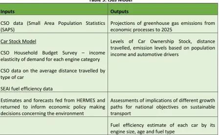
1.2.4 ISus
[image:17.595.71.520.450.727.2]The Irish Sustainable Development Model (ISus) as previously specified, is a specially developed model capable of modelling the impact of economic activity on the environment that can be linked to HERMES through feedbacks from the environment to the macro-economy. Its function therefore is to provide a tool “to assess the implications of different growth paths for national objectives on sustainable developmentand is used to project emissions and resources” (O'Doherty, et al., 2007). An overview of the inputs and outputs of the ISus Model are presented here in Table 3:
Table 3: ISus Model
Inputs Outputs
CSO data (Small Area Population Statistics (SAPS)
Projections of greenhouse gas emissions from economic processes to 2025
Car Stock Model
CSO Household Budget Survey – income elasticity of demand for each engine category CSO data on the average distance travelled by type of car
SEAI fuel efficiency data
Levels of Car Ownership Stock, distance travelled, emission levels based on population income and automotive drivers
Estimates and forecasts fed from HERMES and returned to inform economic policy making decisions concerning the environment
Assessments of implications of different growth paths for national objectives on sustainable transport
Fuel efficiency estimate of each car by its engine size, age and fuel type
13 consumption. This data is then fed into an input-output model that is used to attribute emissions from these sources.
The Car Stock Sub-Model projects future car ownership, it utilizes distance travelled and emissions data based on population, income, other automotive drivers, together with elasticity assumptions (provided by CSO datasets) (Curtis, 2012).
This model is the most substantial and reliable that is readily available, (yet there are plans to estimate a new car ownership model as part of an energy satellite model for COSMO) therefore it has been identified as being the model of interest in relation to the conversion of car usage into carbon emissions in Ireland. The equation to determine the stock of private cars to 2025 utilises three key variables: the level of disposable income in the economy (Y), the number of cars (C) and the population between 15 and 64 (P) (as similarly outlined in the COM of the NTA model).
The A15 equation is as follows:
(𝐴15) ∆ ln
𝐶
0.8
𝑡𝑃
𝑡− 1
= 𝛼 + 𝛽
𝑌
𝑡𝑃
𝑡14
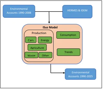
Figure 5: Flowchart of ISus (Devitt et al., 2010)
Lastly, the ESRI Environmental Accounts, which provide trends in emissions and hence highlight areas of concern, are a significant source of information on environmental policy in Ireland that adhere to strict international standards. However the environmental accounts are most useful in projecting the ramifications of policies into the future to test their possible success or failure based on an environmental perspective (Lyons and Tol, 2006).
Critical Analysis of the ISus Model
Pros: Projections of greenhouse gas emissions from economic processes to 2025 are significant in the context of the GDA Draft Transport Strategy for 2030 and as a result, these forecasts will provide substantial support and guidance to the development of our transport emissions model.
The Car Stock Model will be applied in our research in examining the effect of sustainable car usage and reduced car ownership rates. More up to date data will be fed into this model to provide new compelling results.
The synchronisation between HERMES and ISus will prove to be highly significant in the context of Work Package 5 as our analysis of fiscal changes and other economic policies will be tested to study their potential promotion of sustainable car use.
Cons:
Environmental
Accounts 1990-2008 HERMES & IDEM
Environmental Accounts 1990-2025 Cars Energy
Agriculture
Waste Other
Trends Consumption
ISus Model
15 A closer examination of other modes of transport and their carbon emission projections to 2025 is stark limitation of ISus, as public transport, although sustainable in the long term, must be studied in order to increase fuel efficiency and to reduce high emitting vehicles in the fleet (this will be examined in Work Package 4).
1.2.5 UCD MOLAND Model
The MOLAND (Monitoring Urban Land Cover Dynamics) model was developed as part of a European Commission’s Joint Research Centre for assessing and analysing urban and regional development trends across Europe. It was originally developed by RIKS b.v.2 (formerly the University of Maastricht, the Netherlands) and was piloted-tested in 2009 in the GDA using 1990, 2000 and 2006 data (Williams and Convery, 2012). ‘It is the main tool for Land Use Modelling Platform project that supports policy needs of different services of the Commission, for ex-ante assessments and more specific impact assessments’ (Petrov, et al., 2011). Presented in Table 4 are the main inputs and outputs associated with the MOLAND Model:
Table 4: MOLAND Model
Inputs Outputs
Land use maps produced by ERA-Maptec Ltd. County boundary and Electoral Division (ED) maps from Ordnance Survey Ireland (OSI)
Maps of predicted land uses and their locations (analyses quantitatively and spatially)
Transport network – roads and rail datasets from DTO/ NTA and NRA
Illustration of land use change over time which identifies irresponsible planning and zoning of land
Zoning maps developed with protection, conservation and national heritage areas included
Provides a tool to aid understanding of outcomes to specific policies spatially and the effect that this has on transport accessibility Suitability – highly suitable towns map in the
Dublin-Belfast transport corridor used for MD scenario,
-restricted 2km buffer zone along coastline for CD scenario and
- BU and R scenarios a default suitability map used (Petrov et al., 2011).
Planning scenario analysis up to 2026 (Business as Usual (BU); Compact development (CD); Managed Dispersed (MD) and Recession (R))
Socio-Economic data – CSO and ESRI datasets used and extrapolation technique used to generate forecasts
Illustration of socio-economic trends using GIS software
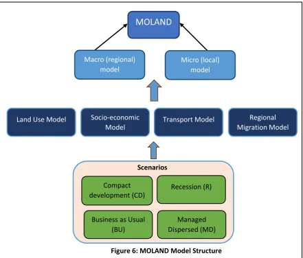
16 MOLAND was implemented in Step 3 of the Strategic Environmental Assessment (SEA) section of the Regional Planning Guidelines (RPGs) of Ireland for which University College Dublin (UCD) assembled an academic research team and UCD have been heavily involved in its development as a tool by applying it to Irish scenarios. The model comprises of 4 interrelated models: (i) a dynamic land use model; (ii) a socio-economic model; (iii) a transport model; (iv) a regional migration model. Accordingly, it has many uses of which the most important is its ability to perform a range socio-economic scenario simulations such as population growth or an increase in un-employment and the assessment of alternative policy options like restrictive zoning plans or per-km car levies (Convery and Williams, 2013). These models are fed into 2 sub-models: the Macro Model (accounts for international trends in population and economic growth and it applies international trends to areas such as the GDA to represent processes like regional migration and urban sprawl) and Micro Model (provides the most detailed account of economic activities in the form of a land use model).
Figure 6: MOLAND Model Structure
The four interrelated model listed above are the instruments used to carry out a range of scenarios based on changing patterns up to year 2026 (similarly in line with NTA, HERMES and ISus model forecast targets) which are influenced by socio-economic trends taken from CSO and ESRI estimates with regards to population, employment and residential configurations. These scenarios as illustrated in Figure 6 above are: Business as Usual (BU); Compact development (CD); Managed Dispersed (MD) and Recession (R) and each of them examine an alternate form of development in the GDA.
Scenarios
MOLAND
Land Use Model Socio-economic
Model Transport Model
Regional Migration Model
Business as Usual (BU) Compact development (CD)
Managed Dispersed (MD)
Recession (R) Macro (regional)
model
Micro (local) model
17 “BU scenario explores the further development of urban patterns emerging before the economic crisis whereas the R scenario focuses on future urban development due to recession, including a recovery by 2016. The CD scenario is important in demonstrating less pressure on natural land uses, exploring urban growth and urban/regional development in the frame of a strong environmental protection policy. In the MD scenario we investigated in more details the growth and sprawl of rural town and villages in open countryside particularly along the Dublin-Belfast motorway” (Petrov et al., 2011).
The main differences that are witnessed between the scenarios are related to population processes such as inward and outward migration in the GDA, both nationally (regional and local scale) and internationally (global scale), as well as the employment figures associated with each of the scenarios. Aspects of employment are particularly significant in the context of transport modelling as employment trends dictate much of what occurs in terms of residential/ urban settlement patterns and centres of employment. Questions such as: Are these locations adequately accessible with strong and reliable links to the transport network? Are commuting patterns in a particular area sustainable? Issues regarding commuting times, public transport priority, infrastructure for active travel modes (walking and cycling) are all highly complex matters which is why new development projects tend to have a large number of stakeholders/ policymakers involved in the process. In response to the outcomes of the proposed scenarios, Petrov et al. (2012) have stated that the highest increase in urban areas in the 2006-2026 period is in MD (269%) and BU (268%) scenarios in County Meath, followed by Wicklow, Kildare and Louth. In 2026 the GDA is estimated to have 9.2% residential, 0.4 commercial, 1.1% industrial and 0.5% service increase in the MD scenario.
Urban development in the GDA has historically been sporadic, poorly controlled and even reckless at times with residential patterns stretching further and further away from large urban zones as a result of an unstable housing market which has resulted in longer commuting times for many people that has a clear and direct knock-on effect on rising car ownership and emissions levels, especially at rush hours. Thus, a model such as MOLAND has been instrumental in assessing hypothetical but highly realistic environmental and land use management situations such as urban form characteristics (density, mixed-use development, proximity to public transport and distance to urban centres) which are vital in the promotion of sustainable development practices. As transport network data is provided by the NTA and NRA much of the information can be examined in greater detail from those sources, the MOLAND model functions as tool to simulate scenarios based on a range of socio-economic being fed into it, and produced GIS based maps to illustrate its outcomes. However, results such as the percentage of urban areas within 1km of transport nodes and the minimum distance of residential areas urban centres are considerably useful to the research aims of the project.
Critical Analysis of the MOLAND Model
Pros:
Provides a tool to aid understanding of outcomes to specific policies spatially and the effect that this has on transport accessibility.
18 MOLAND offers an extensive framework for the comparison of conflicting socio-economic trends up to 2026 (in line with NTA, NRA and ESRI forecasts) and visualises these patterns using GIS software.
The ‘business as usual’ scenario acts essentially as a ‘do minimum’ scenario in relation to current trends which similarly links up well with the NTA and NRA models.
Increasing land density with more mixed-use development is proven to reduce transport-related emissions and by reducing travel to employment and services this could allow for an increased modal shift to public transport or active modes (Williams and Convery, 2012). The MOLAND model supports this agenda which could influence policymakers and stakeholders in coming years.
Cons:
The updated version of MOLAND with the extended transport model was not made available within the time frame of this research undertaken by UCD, the work of populating the transport model with relevant data and associated calibration was preliminary (Williams and Convery, 2012).
Significant data gaps exist that have been highlighted by the MOLAND project team including a lack of harmonised data (both scalar, temporal and contextual) relating to zoning status of lands in the GDA region.
1.3 The Department of Transport, Tourism and Sport (DTTaS) (2016) Common Appraisal
Framework for Transport Projects and Programmes
Supplementary to the transportation models detailed above, it is necessary to consider important transport parameters included in the DTTaS Common Appraisal Framework for Transport Projects and Programmes (DTTaS, 2016). This document was released in March 2016 as a replacement to the Guidance document from 2009, it develops a framework for the evaluation of investments in transport that is also consistent with the Public Spending Code (PSC) to aid in the preparation of business cases of transport investment prior to Government submission (DTTaS, 2016). The document consists of 7 sections each representing a themed issue, the fifth of which will be of specific interest to the Greening Transport Project as it deals with significant transport parameters for use in economic appraisal in examining a project’s broader economic, social and environmental impacts’ (DTTaS, 2016).
19 The range of transport parameter values are displayed in Table 5 below.
Table 5: DTTaS Transport Parameter Values
Parameter Values
Value of Time - Work (hourly labour costs = dividing aggregate labour costs by annual hours worked) - Commuting (10% above the leisure value of time)
- Leisure (40% of average hourly earnings of travellers) Vehicle Operating
Costs
- Fuel Costs (weighted average of Irish road vehicle fleet and applying standard fuel consumption factors by vehicle and road type)
- Non-fuel Costs (oil, tyres, maintenance and depreciation and main vehicle types) Estimated using function C = a1+b1/V,
where: C is cost in cents per kilometre, V is average link speed in km/h, a1 and b1 are parameters for each vehicle category
Emission Values - Noise (€30 per DB(A) per person per year proposed, not definite)
- CO2, NOx and PM (apply rate of emissions per vehicle km, derive total emissions, apply monetary value to each amount of emission from motorways, urban and rural) Active Travel Values - Health Benefits (calculated reductions in risk of death and no. of walkers and cyclists
used to calculate a figure for the potential no. of lives saved based on average mortality rate. No. of potentially prevented deaths multiplied by value of prevented fatality used in accident analysis to give a monetary benefit)
- Absenteeism Benefits (monetary value is the product of the total hours per year saved and value of work time per hour)
Value of time refers to the benefit of travel time savings and this varies according to journey purpose (e.g. work (commuting), education, employer’s Business, shopping, other leisure and non-home based travel as stated in the NTA model). Aggregation of these time savings are calculated to determine the value of such benefits, from 2011 data. The parameters of interest are: Value of Time, Vehicle Operating Costs, Emission Values and Active Travel Values which are explained in Table 5 above.
Future carbon emissions values are set by the Department of Public Expenditure and Reform to 2050. Vehicle emission factors are estimated from the default values contained with the COPERT 4 road transport emissions model and weighted to the Irish vehicle fleet (DTTaS, 2016). A comprehensive analysis of COPERT 4 will be presented in Section 2.2 of this deliverable. From 2015 to 2020 the price of CO2 on the EU ETS system of the European Climate Exchange is used as the cost of CO2 as well as linear extrapolation for carbon price between 2017 and 2020. In the period of 2020 onwards the Impact Assessment from the EU 2030 Framework for Climate and Energy Policy provides a price projection for the ETS. For other gases such as NOx and PM, they are determined by a willingness-to-pay (WTP) valuation method and future values reflect future earnings related to increases in GNP per person employed (DTTaS, 2016).
Active travel benefits and/ or costs are considered by combining benefits from a reduction of health risk and absenteeism as result of increased numbers of people walking and cycling.
20
1.4 International Best Practice - UK, the Netherlands and Sweden
Evidence supporting international best practice in transportation modelling in the context of measuring emission levels will be examined in this section taking case studies of countries in Europe: the United Kingdom, the Netherlands and Sweden, in a comparative analysis. These studies have been suggested based on the range of policy applications that these National Transportation Models present that have been advised by the WSP (2011) report which states that “their use has been central to the development of closer integration with physical and environmental planning of new approaches to transport pricing policy”.
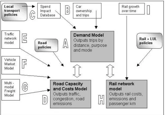
UK National Transport Model (NTM)
Akin to the NTA and NRA models the UK model is an integrated, multi-modal model which is based on the framework of a 10 Year Plan. The model examines car drivers, car passengers, rail, bus, walk and cycle and is comprised of a series of sub-models which are applied in iteration to produce the main model outputs. These models are: the Demand Model, the Road Capacity and Costs Model and the National Rail Model, the functions of which are to produce forecasts of modal share and to examine effect of a change in mode costs due to congestion, road pricing etc. (DtF, 2003). An overview of the model structure is displayed below in Figure 7.
[image:25.595.162.432.371.559.2]The model utilizes data from a wide range of trustworthy sources such as: the National Travel Survey, Family Expenditure Survey, the Traffic Census, ticket sales data as well as the Department of Transport’s National Trip End model data amongst others.
Figure 7: UK NTM Model Structure (DtF, 2003)
21 links directly back to the demand model. The outputs are produced thanks to the volume of data provided from the UK’s Traffic Network Model (highway distribution and assignment) and the Vehicle Market Model (fuel efficiency and vehicle fleet characteristics). Therefore, emissions and transport modelling are interlinked in the FORGE model which is necessary to engender direct coordination.
On the contrary, the ISus Car Stock Model is completely detached from transportation models in Ireland, it is connected to HERMES, and this highlights the fundamental issue that there needs to be greater synchronisation between environmental planning and transport modelling and policy to ensure that environmental policies are adequately enforced to achieve the environmental results. The Greening Transport project proposes to considerably reduce this separation by creating a Transport Emissions model that influences aggregation between these models.
The Netherlands National Model System (NMS)
The Dutch National Model System is a prime example of a highly disaggregate model for predicting travel demand which has been in operation since 1986 and updated on numerous occasions since then. It was originally designed to be a tool for strategic appraisal of new road and rail links but its scope of application has gradually widened to also include environmental and IT issues (Lundqvist and Mattsson, 2001).
The model structure is based upon age-cohort licence holding and car ownership models that are fed into trip frequency, mode and destination choice models. The resultant Origin-Destination rail and car driver trip matrices are then assigned to the rail and road networks. These models are usually based on individual utility maximisation represented in the form of multinomial nested logit models. When applied to forecasting, enumeration of prototypical samples are used together with the ‘pivot-point’ approach for driver and train passenger flows i.e. the model system is only used to calculate changes that are applied to the ‘observed’ based year O/D matrices (Lundqvist and Mattsson, 2001). What sets the NMS apart is the clarity given to the behavioural mechanisms that it implements which in turn means that the model can be deciphered a lot easier. It devotes particular emphasis to Stated Preference (SP) choice modelling to inform the multinomial nested logit models by means of the national travel survey. This technique is unique in that it is designed to infer the maximum amount of information from the survey respondent which is important in the context of demand forecasting using hypothetical situations. For instance in cases where new alternate modes of transport are introduced to the network, a new travel demand will subsequently need to be created to account for this new development. SP presents a useful means of modelling demand for scenarios such as this, which in this way highlights its importance in a transport model and why it should be given more attention (Lundqvist and Mattsson, 2001).
The examination of smarter travel options and opportunities for sustainable car use in Ireland in Work Package 3 and 5, will require an acute analysis of SP modelling to further study and discover opportunities for a shift in behavioural change in the project.
Sweden SAMPERS Model
22 and Gothenburg that focused on transport accessibility, land use and carbon emissions; congestion charges and potential consequences of their introduction as well as in modal demand shifts and route choice decision making processes (Jonsson et al., 2011).
There are five regional models that generate O-D trips in SAMPERS of which nested logit models are used to carry out the estimation of six trip purposes (work, business, school, visits, leisure and other trips) from five modes of transport (car, car passenger, public transport, bicycle and walking). The model inputs time and cost parameters from census data and socio-economic parameters that provide data on car ownership, income and other attraction variables for destinations. The demand model is reliant on matrices from the time and cost parameters that are computed and assigned to traffic/ road and public transport networks in EMME/2 module software (Jonsson et al., 2011). Special software modules such as this have been developed for the design of scenarios, with an automatic control of input data, and for the analysis, aggregation and visualisation of the results (Lundqvist and Mattsson, 2001).
[image:27.595.140.460.434.651.2]SAMPERS like all resource intensive modelling such as transport, it is not free of limitations or errors, and many of such errors become apparent whilst the model is functioning. In a sub-model of SAMPERS entitled SAMKALK that carries out the function of costs and benefits, errors are inadvertently exposed during the functioning of the model. As this sub-model computes CBA the inadequacies in the sensitivity analyses completed elsewhere in SAMPERS as well as quality control features of EMME/2 become apparent. The reason for this is due to the fact that “the sensitivity analyses were not done on model assumptions, only on the CBA assumptions” (Lundqvist and Mattsson, 2001). These errors have been acknowledged by industry partner and other stakeholders, however the model has continued to be used irrespective of this as the model is still very valuable and compares well with state-of-practice. The SAMPERS model structure as depicted by SIKA is display here in Figure 8.
Figure 8: Sweden SAMPERS Model Structure (SIKA, 2002)
Conclusion
23 NTA, NRA and ISus models and provides district recognition of the emissions modelling. Notwithstanding this, elements from the Dutch and Swedish models will also be considered in the development of the transport emissions model and lessons from them will also be taken into careful consideration.
- Learning from the EU examples
[image:28.595.68.513.326.767.2]The bulk of learning potential in terms of the European examples listed can be taken from the UK NTM as it applies specific emphasis to the collaboration of emission modelling with more generalised transport modelling techniques. The gap between these modelling areas must be significantly bridged in Ireland through greater coordination and unification to calculate more accurate GHG emissions from different modes of transport into the future. Lessons can be taken from SAMPERS use of the CBA assumptions mechanism in the Swedish model, especially in planning investment into sustainable modes and taking a longer term perspective. Finally the Dutch model is particularly useful with respect to the incorporation of utility maximisation in multinomial nested logit modelling techniques that may similarly be applied to our transport emissions model in examining travel behaviour. An overview of the key elements from the transportation models discussed is presented in Table 6.
Table 6: Key Elements from the Models
Elements
Models
AM and PM Peak CarbonEmissions & Environmental Concerns Land Use Private Car Ownership TAGM Demand Forecasting Stated Preference Modelling of scenarios NTA GDA
Model
UCD MOLAND
ESRI
HERMES
ESRI ISus
NRA NTpM
UK NTM
Model
The Netherlands
NMS
Sweden SAMPERS
25
Section 2: Examining the most appropriate Environmental Models and Data
2.1 Introduction
Road traffic is one of the greatest contributors to the greenhouse gas (GHG) and reducing it has become one of the main target for sustainable transport policies. Analysis of the main factors influencing GHG emissions is essential for designing environmentally efficient strategies for the road transport. Section 2 describes the review of transportation emission models carried out as a part of Task 2.2.
2.1.1 Classification of emission model
There are various models to calculate emission from road transport which can broadly be classified into Static models (also known as Top-down or Macro-scale emission models) and Dynamic models (also known as Bottom-up or Micro-scale models) (Elkafoury et al., 2014). The Static models can further be classified to Average speed models and Aggregated emission factor models whereas Dynamic models can be sub-classified to Traffic situation model and Instantaneous model. These models have been discussed in the following section.
Average speed model:
These are the most commonly used models which assume that the average emission rate throughout a trip depends on the average speed of the vehicle during that trip. One important drawback of average emission models is that these models don’t allow to calculate emission on spatial resolution but this limitation isn’t much relevant for vehicular emission calculation for vehicle fleet or at national level (Elkafoury et al., 2014). Few examples of average speed models are Computer programme to calculate emissions from road transport (COPERT), Vehicle emissions prediction model (VEPM) etc.
Aggregated emission factor model:
Models of this type operate at the simplest level, with a single emission factor being used for a broad category of vehicles and a general driving condition such as, urban roads, rural roads etc. (Wang and McGlinchy, 2009). These models calculate vehicular emission on the basis of amount of fuel consumed and vehicle kilometre travelled (VKT) (Elkafoury et al., 2014). A few examples of this type of model are the Mobile Source Emission Factor Model (MOBILE), National Atmospheric Emission Inventory (NAEI) etc.
Traffic situation model:
In this type of modelling approach, driving dynamics is also taken into account along with average speed. Traffic situations are defined by traffic conditions (e.g. congested, free flow, stop and go etc.) on a specific type of road such as, urban, along with the speed limit value on that particular road (Wang and McGlinchy, 2009). One issue with this type of model is that it requires detailed statistics about vehicle speed and traffic situation associated with the trips (Elkafoury et al., 2014). Examples of traffic situation models are Handbook emission factors for road transport (HBEFA), Assessment of road transport emission model (ARTEMIS) and Vehicle fleet emission model (VFEM) etc.
Instantaneous model:
26 Table 7 shows the input data required to define the vehicle operation, characteristics and area of application of the above mentioned transportation emission models.
Table 7: Emission models (Ref. NZ Transport Agency, 2013)
Type Input data required to
define vehicle operation
Characteristics Application
Aggregated emission factor model
Area or road type Simplest level, no speed or vehicle specific dependency
National inventories
Average speed model
Average trip speed Speed and vehicle type/ technology specific
National and regional inventories
Traffic situation Model
Type of road, speed limits, congestion level
Driving pattern (speed, acceleration etc.) and vehicle type/technology specific Environmental impact assessment, area-wide urban traffic management (UTM) assessment Instantaneous Model
Driving pattern, vehicle specific data- power, speed etc.
Micro-scale modelling, individual vehicle specific
UTM assessment
2.2 The existing emission modelling tools
This section gives brief summary of various models developed to calculate emission from road transport. Apart from models which has been developed by European countries, models developed in USA and New Zealand has also been included. Table 8 presents advantages and disadvantages of all the important transportation emission models.
2.2.1 Assessment of Road Transport Emission Model (ARTEMIS)
ARTEMIS is a Traffic Situation model (André et al., 2004). This is one of the most comprehensive transportation emission models and it can operate at both macro and micro level (Wang and McGlinchy, 2009).
27 ARTEMIS can calculate emission for road, rail, air and ship transport and provides consistent emission estimates at both national and regional level. The ARTEMIS tools were designed for three main applications, emission inventories, scenario calculation for assessing the impacts of alternative measures and inputs for air quality models in order to assess spatial and temporal impacts on the environment (UNECE Transport Division report, 2012). The model has many similarities with COPERT and HBEFA models (these models have been discussed on the following two sections), especially in terms of input vehicle classes and categories of GHG and air pollutants to be obtained as output. For emissions from light vehicles, ARTEMIS have improved emission factors than COPERT and HBEFA (Wang and McGlinchy, 2009).
As per UNECE Transport Division report (2012), ARTEMIS has only been fully implemented for compiling national air emission inventories in four countries, i.e. Germany, Austria, Switzerland and Sweden. Application of the model to other countries is not possible without the involvement of the ARTEMIS modelling team.
2.2.2 Computer Programme to Calculate Emissions from Road Transport (COPERT)
COPERT is an Average Speed model. COPERT has been developed for official road transport emission inventory preparation for European Environment Agency (EEA) member countries (Austria, Belgium, Bulgaria, Croatia, Cyprus, Czech republic, Denmark, Estonia, Finland, France, Macedonia, Germany, Greece, Hungary, Iceland, Ireland, Italy, Latvia, Lithuania, Luxembourg, Malta, Netherland, Norway, Poland, Portugal, Romania, Slovakia, Slovenia, Spain, Sweden, Switzerland, Turkey, United kingdom) (EMISIA, 2014). COPERT 4 is the most modified and latest available version of COPERT which took elements from few other popular emission models like, MEET, ARTEMIS, COST and PARTICULATES. Its initial version was COPERT 85 (1989), followed by COPERT 90 (1993), COPERT II (1997) and COPERT III (1999). COPERT 4 (2006). COPERT II was the first one with a GUI (Graphical Use Interface), built on MS Access 2. COPERT II provided emission factors up to Euro 1. COPERT III was based on menus and compared to COPERT II, it has new features like, hot emission factors for Euro 1 passenger cars, reduction factors over Euro 1 according to AutoOil, Impact on emissions from 2000, 2005 fuel qualities, Cold-start methodology for post Euro 1 Passenger cars (PC), Emission degradation due to mileage, Alternative evaporation methodology, Detailed NMVOC (Non-methane Volatile Organic Compounds speciation (Polycyclic Aromatic Hydrocarbon (PAH)), Persistent Organic pollutants (POP), Dioxins and Furans), Updated hot emission factors for non regulated pollutants. COPERT 4 can calculate emission from a wide range and variety of vehicles e.g. Hybrid passenger cars, Compressed Natural Gas (CNG) buses, Liquefied Petroleum Gas (LPG) passenger cars, conventional heavy duty vehicles in addition to the conventional diesel vehicles. Three types of roadway situations can be considered in COPERT i.e. Urban, Rural and Motorways. The shortcoming about heavy vehicle (>13T) emission in NAEI is improved in COPERT and it gives more reliable results for emissions from heave vehicle as it is tested on more no. of vehicles. COPERT 4 includes many important emission factors such as, cold over hot ratio, ambient temperature, vehicle use, mileage, fuel characteristics etc. For heavy vehicles, loading and gradients are also taken into account. The latest version of COPERT i.e. COPERT 5 will be launched in September, 2016 (EMISIA, 2015). Street level COPERT is also available which calculates only hot emissions with at street level and can be combined with meso and macro emission models (Dilara, 2015).