Implementing Semantic Query Optimization in Relational Databases

ABSTRACT

Semantic query optimization is applied to relational databases using the inductive learning approach. This approach generates an alternate query using the learning framework and the algorithm. The alternate query should be semantically equivalent to original query. The semantically equivalent query generated should be less expensive than the original query. These can be implemented in SQL using the SQL hints. These hints allow user to implement the desired plan for the query.

Keywords

Semantic query; semantic query optimization; SQL hints; inductive learning; algorithm for learning; learning framework

1.

INTRODUCTION

A semantic query is a query pertaining to knowledge or data that is expressed purely on the basis of a common business vocabulary, without any reference to how or where the data is stored. Semantic query refers to database queries that are based on concepts, properties and instances defined in an ontology and that return semantically relevant results. A semantic query attempts to help a user to obtain or manipulate data in a database without knowing its detailed syntactic structure. For example, the query: "list the name of all employees in the database" is semantically equivalent to the syntactic query: "list the name of all faculty, trainee and employee in the database", provided the database semantics specify that all faculty members and trainees are employees [8, 10 and 12]. The term Semantic Query Optimization refers to the process of utilizing the integrity constraints in the optimization process. The underlying concept of semantic query optimization is that by harnessing the integrity constraints, a user’s query can be transformed into a query which is syntactically different to the original but which will produce the same result for all states of the database, and be more efficient to execute than the original query [2]. Semantic query optimization results in the transformation of an input query into a “semantically equivalent query”. Two queries are

said to be semantically equivalent if, for every state of the database, they produce the same result. Semantic query optimization in relational databases can be done by using the concept of inductive learning. It can be implemented in SQL using the SQL hints [1, 3].

2.

INDUCTIVE LEARNING

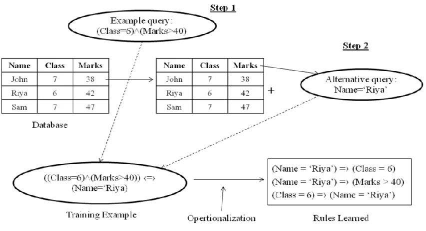
Figure 1. Learning Framework for Inductive Learning Approach

An algorithm is defined to generate the alternate query that is semantically equivalent to the original query. The input of the algorithm is a user query Q and the database relations DB. The primary relation of a query is the relation that must be accessed to answer the input query. Initially, the system determines the primary relation of an input query and labels the instances in the relation as positive or negative. An instance is positive if it satisfies the input query; otherwise, it is negative [7].

Algorithm –

INPUT Q = input query; DB = database relations; BEGIN

LET r = primary relation of Q; LET AQ= alternative query (initially empty);

LET C = set of candidate constraints (initially empty);

Construct candidate constraints on r and add them to C;

REPEAT

Evaluate gain/cost of candidate constraints in C;

LET c = candidate constraint with the highest gain/cost in C;

IF gain(c) > 0 THEN

Merge c to AQ, and C = C - c; IF AQ Q THEN RETURN AQ;

IF c is a join constraint on a new relation r' THEN

Construct candidate constraints on r' and add them to C;

UNTIL gain(c) = 0;

RETURN fail, because no AQ is found to be equivalent to Q;

END.

The algorithm initially takes an input query Q, database DB, primary relation of input query r, an empty alternate query AQ and an empty set of candidate constraints C. A candidate constraint is created on r and is added to set of constraints C. The gain/cost of candidate constraints is evaluated. The constraint with the highest gain/cost ratio is stored in c. If the gain of c is greater than 0, the candidate constraint is merged with alternate query AQ and is removed from the set of candidate constraints C. If the AQ is found equivalent to Q, the value of AQ is returned. Next c is checked whether it is a join constraint on a new relation r'. If it is a join constraint on r' then candidate constraints on r' are constructed and are

added to

C. This whole process is continued till the gain value of c becomes zero. If no AQ equivalent to Q is found, algorithm returns fail and the algorithm ends.

3.

SQL HINTS

each component query, then hints in the first component query apply only to its optimization, not to the optimization of the second component query.

You can use hints to specify the following:

 The optimization approach for a SQL statement

 The goal of the cost-based optimizer for a SQL statement  The access path for a table accessed by the statement  The join order for a join statement

 A join operation in a join statement

Hints provide a mechanism to direct the optimizer to choose a certain query execution plan based on the following criteria:  Join order

 Join method  Access path  Parallelization

4.

EXPERIMENTAL RESULTS

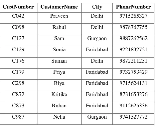
We take a Bank database having tables placed on same location. The Bank database has three tables – CustomerDetail and Account. The CustomerDetail table stores the information of the customer like the customer name, city of customer and phone number. The Account table have information of the account like account number, ID of account holder, branch city where account exists and balance in the account. These tables are shown below.

Table 1. CustomerDetail

CustNumber CustomerName City PhoneNumber

C042 Praveen Delhi 9715265327

C098 Rahul Delhi 9878767755

C127 Sam Gurgaon 9887262562

C129 Sonia Faridabad 9221832721

C176 Suman Delhi 9872211231

C179 Priya Faridabad 9732753429

C298 Riya Faridabad 9715624131

C872 Kritika Faridabad 8731653276

C873 Rohan Faridabad 9112625336

C987 Neha Gurgaon 9741327772

We query the database to retrieve the account number, customer name and balance of those accounts which have CustNumber < ‘C200’ and the BranchCity of Account is same as City of Customer from the CustomerDetail and Account table. The SQL query for this would be –

Query 1: Select the account number, customer name and balance in account where the owner ID of Account table is same as customer number, customer number is less than C200 and the BranchCity of Account is same as City of Customer from the Account table and CustomerDetail table.

SQL Query –

Select AccountNumber, CustomerName, Balance From Account as A, CustomerDetail as CD

Where A.OwnerID=CD.CustNumber and

CustNumber<'C200' and BranchCity=City

The query can be executed in different ways. In centralized database, the join technique used for joining the tables plays the most important role as the join method can reduce or increase the size of the plan and the query cost. So we implement different join methods and see the difference between each. The joins are implemented using SQL hints. Plan 1 –

Using inner loop join on CustomerDetail and Account tables. The SQL hint used for this is ‘inner loop join’. The query looks like –

Select AccountNumber, CustomerName, Balance

From Account as A inner loop join CustomerDetail as CD on A.OwnerID=CD.CustNumber

Where CustNumber<'C200' and BranchCity=City

The query execution plan for plan 1 is shown below in figure 2.

A632 C129 Faridabad 80000

A634 C179 Faridabad 45000

A675 C298 Faridabad 25000

A7162 C098 Delhi 72000

A721 C987 Gurgaon 20000

A723 C176 Gurgaon 25000

A761 C298 Faridabad 35000

A932 C129 Gurgaon 40000

A981 C872 Faridabad 25000

Figure 2. Query plan 1 for Query 1

Plan 2 –

Using merge on CustomerDetail and Account tables. The SQL hint used for this is ‘inner merge join’. The query looks like –

Select AccountNumber, CustomerName, Balance

From Account as A inner merge join CustomerDetail as CD on A.OwnerID=CD.CustNumber

Where CustNumber<'C200' and BranchCity=City

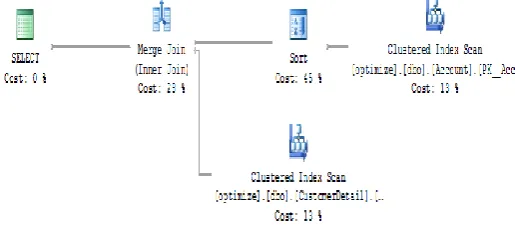
The query execution plan for plan 2 is shown below in figure 3.

Figure 3.Query plan 2 for Query 1

Plan 3 –

Using right outer hash join on CustomerDetail and Account tables. The SQL hint used for this is ‘right outer hash join’. The query looks like –

Select AccountNumber, CustomerName, Balance

From Account as A right outer hash join CustomerDetail as CD on A.OwnerID=CD.CustNumber

Where CustNumber<'C200' and BranchCity=City

The query execution plan for plan 3 is shown below in figure 4.

Figure 4. Query plan 3 for Query 1

Plan 4 –

Using left outer hash join on CustomerDetail and Account tables. The SQL hint used for this is ‘left outer hash join’. The query looks like –

Select AccountNumber, CustomerName, Balance

From Account as A left outer hash join CustomerDetail as CD on A.OwnerID=CD.CustNumber

Where CustNumber<'C200' and BranchCity=City

The query execution plan for plan 4 is shown below in figure 5.

Figure 5. Query plan 4 for Query 1

We now compare these plans for Query 1. The comparison is done on basis of three criteria – cached plan size, relative query cost and estimated query cost.

Table 3. Comparison of query plans for Query 1

Plan number

Cached Plan Size (in Bytes)

Relative Query Cost

(in %)

Estimated Query Cost

(in sec)

1 13 9 0.0075697

2 21 31 0.0254061

3 35 30 0.02464324

same as customer number and balance in account is greater than 40000 from the Account table and CustomerDetail table.

SQL Query –

Select AccountNumber, CustomerName, Balance From Account as A,CustomerDetail as CD

Where A.OwnerID=CD.CustNumber and Balance>40000 Different execution plans for query 2 are defined as follows. Plan 1 –

Using inner loop join on CustomerDetail and Account tables. The query looks like –

Select AccountNumber, CustomerName, Balance

From Account as A inner loop join CustomerDetail as CD on A.OwnerID=CD.CustNumber

Where Balance>40000

The query execution plan for plan 1 is shown below in figure 6.

Figure 6. Query plan 1 for Query 2

Plan 2 –

Using merge on CustomerDetail and Account tables. The query looks like –

Select AccountNumber, CustomerName, Balance

From Account as A inner merge join CustomerDetail as CD on A.OwnerID=CD.CustNumber

Where Balance>40000

The query execution plan for plan 2 is shown below in figure 7.

Figure 7. Query plan 2 for Query 2

Plan 3 –

Using right outer hash join on CustomerDetail and Account tables. The query looks like –

Select AccountNumber, CustomerName, Balance

From Account as A right outer hash join CustomerDetail as CD on A.OwnerID=CD.CustNumber

Where Balance>40000

The query execution plan for plan 3 is shown below in figure 8.

Figure 8. Query plan 3 for Query 2

Plan 4 –

Using left outer hash join on CustomerDetail and Account tables. The query looks like –

Select AccountNumber, CustomerName, Balance

From Account as A left outer hash join CustomerDetail as CD on A.OwnerID=CD.CustNumber

Where Balance>40000

The query execution plan for plan 4 is shown below in figure 9.

We now compare these plans for Query 2. The comparison is done on basis of three criteria – cached plan size, relative query cost and estimated query cost.

Table 4. Comparison of query plan for Query 2

Plan number Cached Plan Size (in Bytes) Relative Query Cost (in %) Estimated Query Cost (in sec)

1 10 9 0.0072389

2 14 31 0.0250769

3 27 30 0.0245428

4 26 30 0.0245427

As it is shown in table 4 that the plan 1 not only has less cost as compared to other plans but it also had less cached plan size. So plan 1 is found to be most optimum execution plan for Query 2. Thus, plan 1 will be used to process Query 2. Now we compare the optimized plans of query 1 and query 2. By comparing the optimized plans of both queries we get the best query to be used for processing the query for the same result.

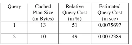
Table 5. Comparison of optimized plans of query 1 and Query 2

Query Cached Plan Size (in Bytes) Relative Query Cost (in %) Estimated Query Cost (in sec)

1 13 51 0.0075697

2 10 49 0.0072389

Table 5 shows that the query 2 is more efficient than query 1. Query 2 have less cached plan size and relative and estimated cost. Thus the query 2 can be used instead of query 1 so that the cost and size for query is reduced.

5.

CONCLUSION

The semantically equivalent query generated using the inductive learning method is more efficient than the original query fired by the user. This is clear from the table 5. Table 5 clearly shows that even the best plan for the original query is less efficient than the best plan of the semantically equivalent query. The inductive learning method not only reduces the cost of execution of query but also reduces the size of plan used while executing the query. The concept of semantic query optimization proves to be beneficial in optimizing the queries.

The semantic query optimization can further be extended to the distributed databases. In distributed databases not only optimization is difficult but also the query processing is complicated as compared to the relational databases. The semantic query optimization will be more difficult to be implemented in distributed databases as the databases are stored at different locations. So the generation of alternate query will not be an easy process. A very different and strong

semantically equivalent query in distributed databases. The algorithm should be able to take data from the different site and generate an alternate query for the original query fired. The alternate query should be semantically equivalent and less expensive.

6. REFERENCES

[1] Bruno Nicolas, Chaudhuri Surajit and Ravishankar Ramamurthy, “Power Hints for Query Optimization”; In Proceedings of the International Conference on Data Engineering (ICDE), IEEE, 2009.

[2] Cardiff J, “The Use of Integrity Constraints to Perform Query Transformations in Relational Databases”; Proc. PARBASG 90, IEEE Computer Society Press, 1990. [3] Cardiff J. and M. Orlowska, “A Geometric Approach to

Semantic Query Optimisation in Relational Databases”; Proc. of the Fifth Int. Symposium on Methodologies for Intelligent Systems, Elsevier Publishing Co., 1990. [4] Carlos Ordonez, “Optimization of Linear Recursive

Queries in SQL”; IEEE Transactions on Knowledge and Data Engineering, Vol. 22, No. 2, page(s): 264-277, February 2010.

[5] Hsu C. and C. A. Knoblock, “Rule induction for semantic query optimization”; In Proc. 11th International Conference on Machine Learning, pages 112–120, Morgan Kaufmann, 1994.

[6] Hsu C. and C. A. Knoblock, “Semantic query optimization for query plans of heterogeneous multidatabase systems”; Knowledge and Data Engineering, 12(6):959–978, 2000.

[7] Hsu C. and C. A. Knoblock, “Using inductive learning to generate rules for semantic query optimization”; In Advances in Knowledge Discovery and Data Mining, pages 425–445. 1996.

[8] Kumar P. Mohan and J. Vaideeswaran, “Semantic based Efficient Cache Mechanism for Database Query Optimization”; International Journal of Computer Applications Volume 43– No.23, page(s): 14-18, April 2012.

[9] Panus Jan and Josef Pirkl, “Testing of Oracle database utilization”; International Journal of Applied Mathematics and Informatics, Issue 3, Vol. 4, page(s): 58-65, 2010.

[10]Saini Mayank, Sharma Dharmendar and P. K. Gupta, “Enhancing Information Retrieval Efficiency Using Semantic-based-Combined-Similarity-Measure”; International Conference on Image Information Processing (ICIIP 2011), IEEE Computer Society, 2011. [11]Taniar D., Khaw H.Y., Tjioe H.C. and J.W. Rahayu, “The use of hints in object-relational query optimization”; International Journal of Computer Systems Science and Engineering 19(6), page(s): 337-346, 2004.