Comparison of different Radio Propagation Models with and without Black Hole Attack on AODV Routing Protocol in MANET

Comparison of different Radio Propagation Models with

and without Black Hole Attack on AODV Routing

Protocol in MANET

Abhinav Mehta

PG Scholar Department of ECE

MIT, Mandsaur

Rohit Jain

PG Scholar Department of ECE

MIT, Mandsaur

Vinay Somani

Lecturer Department of ECE

MIT, Mandsaur

ABSTRACT

A Mobile ad-hoc network (MANET) is a temporary network set up by wireless mobile computers (or nodes) moving arbitrary in the places that have no network infrastructure. In this paper the AODV routing protocol in MANET will be discussed. Also various security threats on MANET will be discussed with our major concern on the Black Hole attack . In the later part of this paper there is a description of different radio propagation models and then compare their performance on AODV, with and without Black Hole attack.

Keywords

AODV, MANET, Black Hole.

1.

INTRODUCTION

Mobile ad-hoc networks are composed of autonomous nodes that are self- managed without any infrastructure. Ad hoc networks follow dynamic topology such that any node can join or leave the network at any time. Mobile Ad hoc Networks (MANETs) have become increasingly popular in many applications including emergency search and rescue operations due to their ease of installation and low setup cost, and more importantly their support for users’ mobility Ad-hoc networks are also suitable for areas where it is not possible to set up a fixed infrastructure [1]. In MANETs nodes offer connections by using different routing protocols including Ad-hoc on demand distance vector (AODV), Dynamic source routing (DSR), Destination sequenced distance vector (DSDV) etc. The AODV is one of the widely used routing protocols in MANETs. However, due to various security issues of the routing protocols, wireless ad-hoc networks are vulnerable to attacks of the malicious nodes. One of these attacks is the Black Hole Attack. In this paper different types of attacks are highlighted and the black hole attack is described in the later section.

1.1 Ad-hoc on demand distance vector (AODV)

The AODV routing protocol one of the reactive routing protocol therefore, routes are determined only when needed. When a source node wants to send a message packet to some destination node and does not already have a valid route to that destination, it initiates a route discovery process to locate the other node. It broadcasts a route request (RREQ) packet to its neighbors, which then forward the request to their neighbors, and so on, until either the destination or an intermediate node with a “fresh enough” route to the destination is located. When the RREQ message packet either reaches the destination node or encounters a node with a route to the destination a response

is transmitted. That response occurs via the transmission of a route reply (RREP) message. In case if a node realizes that the route is damaged or broken it transmits a route error (RERR) message to the source [2].

2.

SECURITY ISSUES FOR MANETS

Ad-hoc networks are more vulnerable than wired networks therefore security is much more difficult to maintain in mobile ad hoc networks. Following are the various vulnerabilities that exist in wireless ad-hoc networks: [3]

Open Medium - Eavesdropping is easier than in wired network as there is no centralized medium.

Dynamically Changing Network Topology – Mobile Nodes comes and goes from the network. They dynamically change their topology. This allows any malicious node to join the network without being detected.

Cooperative Algorithms - The routing algorithm of MANETs requires mutual trust between the neighbor nodes which violates the principles of Network Security.

Lack of Centralized Monitoring – There is absence of any centralized infrastructure that prohibits any monitoring agent in the system.

Lack of Clear Line of Defense - In addition to prevention, we need two line of defense i.e. detection and response. Realizing security in ad hoc environments is exceedingly difficult since many different types of ad hoc networks exist. Any variation is possible ranging from predominantly static sensor networks to highly mobile vehicular network scenarios. So, it is necessary to design specialized security solutions adapted to the underlying ad hoc network. Not only the network architecture has to face security threats, also the services and protocols used within the network have to withstand many different attacks.

Following are the different types of attack:-

 Black hole attack  Passive Eavesdropping

 Selective existence (Selfish Nodes)  Gray hole attack (Routing Misbehavior)  Impersonation

 Rushing attack

 Resource consumption attack  Location disclosure attack

3.

BLACK HOLE ATTACK

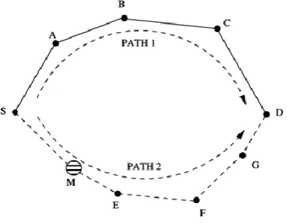
A black hole is a malicious node that incorrectly replies the route requests that it has a fresh route to destination and then it drops all the receiving packets. The damage will be serious if malicious nodes work together as a group. This type of attack is called cooperative black hole attack. The difference of Black Hole Attacks compared to Gray Hole Attacks is that malicious nodes never send true control messages initially.To carry out a black hole attack, malicious node waits for neighboring nodes to send RREQ messages. When the malicious node receives an RREQ message, without checking its routing table, it immediately sends a false RREP message giving a route to destination over itself, assigning a high sequence number to settle in the routing table of the victim node, before other nodes send a true one. Therefore requesting nodes assume that route discovery process is completed and ignore other RREP messages and begin to send packets over malicious node.[1]

Figure 1: Illustration of Black Hole Attack

Figure-1 shows the black hole attack. When a malicious node M enters the network it advertises that it has the shortest path to the destination node D when it receives the Route Request packets sent by node S. The attacker may not be able to succeed if node A, which also receives the Route Request packet from node S, replies earlier than node M. But a major advantage for the malicious node is that it does not have to search its routing table for a route to the destination.

Also, the Route Reply packets originate directly from the malicious node and not from the destination node. Hence, the malicious node would be able to reply faster than node A, which would have to search its routing table for a route to the destination node M, allowing node M to listen all packets meant for destination node.

4. RADIO PROPAGATION MODELS

Radio channels are much more complicated to analyze than wired channels. Their characteristics may change rapidly and randomly [8]. There are large differences between simple paths with line of sight (LOS) and those which have obstacles like buildings or elevations between the sender and the receiver (Non Line of Sight (NLOS)). To implement a channel model generally two cases are considered: large-scale and small-scale propagation models. Large scale propagation models account

for the fact that a radio wave has to cover a growing area when the distance to the sender is increasing. Small scale models (fading models) calculate the signal strength depending on small movements or small time frames. In this paper, three frequently used models for the ns-2 (network simulator-2) are described in more detail.

4.1 Free Space Model

This is a large scale model. The received power is only dependent on the transmitted power, the antenna’s gains and on the distance between the sender and the receiver. It accounts mainly for the fact that a radio wave which moves away from the sender has to cover a larger area. So the received power decreases with the square of the distance. The free space propagation model assumes the ideal propagation condition that there is only one clear line-of-sight path between the transmitter and receiver. H. T. Friss presented the following equation to calculate the received signal power in free space at distance d from the transmitter.[4][5][6][7]

Pr(d) = (PtGtGrλ2) ((4π)2d2L) …………(i)

Where Pt is the transmitted signal power, Gt and Gr are the

antenna gains of the transmitter and the receiver respectively. L (L 1) is the system loss, and λ is the wavelength. It is common to select Gt=Gr=1and L=1 in ns simulations.

4.2 Two Ray Ground Model

The Two Ray Ground model is also a large scale model. It is assumed that the received energy is the sum of the direct line of sight path and the path including one reflection on the ground between the sender and the receiver. A limitation in ns-2 is that sender and receiver have to be on the same height. It is shown that this model gives more accurate prediction at a long distance than the free space model. [4][5][6][7] The received power at distance d is predicted by:

Pr(d) = (PtGtGrht2hr2) (d4L) …………(ii)

Where ht and hr are the heights of transmit and receive antennas

respectively. To be consistent with the free space model L is added here. The above equation shows a faster power loss than Eqn. (i) as distance increases. However, the two-ray model does not give a good result for a short distance due to the oscillation caused by the constructive and destructive combination of the two rays. Instead, the free space model is still used when d is small.

4.3 Shadowing model

The shadowing model of ns-2 realizes the lognormal shadowing model. It is assumed that the average received signal power decreases logarithmically with distance. A Gaussian random variable is added to this path loss to account for environmental influences at the sender and the receiver. The shadowing model consists of two parts. The first one is known as path loss model, which also predicts the mean received power at distance d, denoted by Pr(d). It uses a close-in

distance d0 as a reference. Pr(d) is computed relative to Pr(d0) as

follows.

Pr(d0) Pr(d) =(d/d0)β ………..(iii)

becomes larger. Pr(d0) can be computed from eqn.(i). The path

loss os usually measured in dB.

[Pr(d) Pr(d0)] = -10β log (d/d0) ………. (iv)

The second part of the shadowing model reflects the variation of the received power at certain distance. It is a log-normal random variable that is; it is of Gaussian distribution if measured in dB. The overall shadowing model is represented by

[Pr(d) Pr(d0)] = -10β log (d/d0) +XdB ……… (v)

Where XdB is a Gaussian random variable with zero mean and standard deviation σdB. σdB is called the shadowing

deviation, and is also obtained by measurement. Table.2 shows some typical values of σdB. Eqn. (v) is also known as a

log-normal shadowing model.[4][5][6][7]

Table.1- Some typical values of β.

Environment Β

Outdoor Free Space 2

Shadowed urban area 2.7-5

In Building

Line of sight 1.6-1.8

Obstructed 4-6

Table.2- Some typical values of Standard deviation σdB.

Environment σdB

Outdoor 4-12

Office, hard partition 7

Office, soft partition 9.6

Factory, line of sight 3-6

Factory, obstructed 6.8

5.

SIMULATION ENVIRONMENT

5.1 Simulation Parameters

The simulation has been performed on Network Simulator version 2.35 (NS-2.35). Simulation on AODV routing protocol has been done considering both cases i.e. with Black hole attack and without Black hole attack. Also simulation of three different radio propagation models is done in ns-2.35 whose performance have been compared in both the cases to get the most suitable model for the simulation parameters and scenarios which we have taken. Table 3 shows our simulation environment.

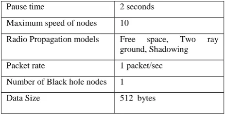
Table.3-Simulation Parameters

Simulation Area 500 X 500, 1000X1000

1500x1500,2000x2000

Number of nodes 20

Communication traffic CBR

Maximum no. of connections 15

Simulation Duration 200 seconds

Pause time 2 seconds

Maximum speed of nodes 10

Radio Propagation models Free space, Two ray ground, Shadowing

Packet rate 1 packet/sec

Number of Black hole nodes 1

Data Size 512 bytes

5.2 Performance Metrics

5.2.1 Packet Delivery Fraction (PDF)

The packet delivery ratio in this simulation is defined as the ratio between the numbers of packets received by the CBR sink at destination to the number of packets sent by sources.

PDF =

5.2.2 End-to-end delay

The average time taken by the packets to pass through the network is called end-to-end delay. This is the time when a sender generates the packet and it is received by the application layer of destination, it is represented in seconds. This is the whole time that includes all delay of network such as transmission time, buffer queues, MAC control exchanges and delay produced by routing activities.

6.

SIMULATION RESULTS

The analysis of simulation results is performed based on the standard metrics of Packet delivery fraction (PDF), End to end (E2E) delay over different radio propagation models. Simulation area is the main parameter which is being varied in the simulations. Also the simulation results have been divided into two different subsections i.e. with black hole attack and without black hole attack.

(a) With black hole attack

(b) Without black hole attack

Figure 2- Comparison of various Radio Propagation models on the basis of PDF varying simulation area.

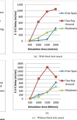
Figure 3 shows the End to End delay of the three models varying simulation area. By analyzing figure 3(a) & 3(b) it can be concluded that the average end to end delay in two ray ground is very high as compared to both the free space and shadowing models of radio propagation. These high delay leads to the small PDF of the two ray ground as shown in figure-1. It can also seen that the free space and shadowing models go neck to neck as far as end to end delay is concerned with free space offering a more delay at 1000 and 2000 m distance.

(a) With black hole attack

(b)

(c) Without black hole attack

Figure 3- Comparison of various Radio Propagation models on the basis of End to End Delay varying simulation area.

7.

CONCLUSION

In this paper it has been tried to analyze the performance of three major radio propagation models. The MANET protocol considered here is AODV and a malicious attack known as black hole attack has also been considered. The simulations have been performed considering both the cases i.e. with black hole and without black hole attack. We demonstrated that the usage of more accurate radio propagation model changes simulated topologies considerably between commonly used propagation models. Consequently, different performance evaluation results have been obtained. Comparison of radio propagation models has been done on the basis of Packet delivery fraction and End to end delay. It is noticed that the black hole attack has a huge impact on the network performance. The PDF of all the models drops heavily in case of black hole attack. The results may vary in the realistic simulation environment where the obstacles such as buildings will lead to the signal fading which will also affect the performance of the different propagation models.

0 5 10 15 20 25 30 35 40

500 1000 1500 2000

PD

F (%

)

Simulation Area (metres)

Free Space

Two Ray Ground

Shadowing

0 20 40 60 80 100 120

500 1000 1500 2000

PD

F (%

)

Simulation Area (metres)

Free Space

Two Ray Ground

Shadowin g

0 200 400 600 800 1000 1200

500 1000 1500 2000

E

-2

-E

D

e

lay

(m

/sec

)

Simulation Area (metres)

Free Space

Two Ray Ground Shadowing

0 200 400 600 800 1000 1200 1400 1600 1800

500 1000 1500 2000

E-2

-E

D

e

lay

(m

/sec

)

Simulation Area (Metres)

Free Space

Two Ray Ground

8. REFERENCES

[1] A. Vani ECE Department CBIT-Hyderabad D. Sreenivasa Rao Professor ECE. Department, JNTU Hyderabad, Andhra Pradesh, India “Removal of Black Hole Attack in Ad Hoc Wireless Networks to provide confidentiality security service”.

[2] C. E. Perkins and E. M. Royer, “Ad-hoc On-Demand Distance Vector Routing,” Proc. 2nd IEEEWksp. Mobile Comp. Sys. and Apps., Feb. 1999, pp. 90–100.

[3] Akanksha Saini, Harish Kumar Department of Computer Science & Engineering, UIET, Punjab University Chandigarh, “Effect Of Black Hole Attack On AODV Routing Protocol In MANET”.

[4] Ingo Gruber, Oliver Knauf and Hui Li,” Performance of Ad Hoc Routing Protocols in Urban Environments”, In Proceedings of European Wireless 2004 (EW'2004, Barcelona, Spain, February 24 - 27, 2004, Barcelona, Spain

[5] http://www.cubinlab.ee.unimelb.edu.au/~jrid/Docs/ Manuel-NS2/node196.html.

[6] www.isi.edu/~weiye/pub/propagation_ns.pdf.

[7] Arne Schmitz, Martin Wenig ,”The Effect of the Radio Wave Propagation Model in Mobile Ad Hoc Networks”,Torremolinos,Malga,Spain,MSWiM’06,Octob er 2-6,2006

[8] www.isi.edu/nsnam/ns/tutorial Marc Greis tutorial on ns2.

[9]